A Coordinated Electric System Interconnection Review—the utility’s deep-dive on technical and cost impacts of your project.
Challenge: Frequent false tripping using conventional electromechanical relays
Solution: SEL-487E integration with multi-terminal differential protection and dynamic inrush restraint
Result: 90% reduction in false trips, saving over $250,000 in downtime
The three operating regions you have to design to
| Device | Output vs voltage | Response | Best suited to | Main limitations |
|---|---|---|---|---|
| Mechanically switched capacitor or reactor | Proportional to voltage squared | Seconds; discrete steps; limited switching operations per day | Steady-state reactive supply, voltage profile, loss reduction | No dynamic capability; step voltage change on switching; capability collapses when most needed |
| Static var compensator | Capacitive branches proportional to voltage squared | A few cycles; continuously controllable | Continuous control where cost matters and deep voltage support is not the driver | Square-law capability loss; harmonic filters are part of the plant and interact with the network |
| STATCOM | Approximately proportional to voltage — constant current capability | One to two cycles closed loop; converter response faster still | Voltage stability margin, weak interconnections, fast disturbance recovery, flicker and unbalance compensation | Higher capital cost; converter losses; adds a converter and its control dynamics to the network |
| Synchronous condenser | Governed by machine capability and excitation | Excitation response in the hundreds of milliseconds; inherent inertial response instantaneous | System strength and inertia, short-circuit contribution, black start support | Rotating plant with maintenance and losses; slower controlled response than a converter |
| STATCOM with energy storage | Reactive as a STATCOM, plus real power within the storage rating | As STATCOM for reactive; real power limited by storage | Where a real power deficiency is part of the problem | Cost and complexity of the storage; different failure and maintenance profile |
| Service area | What we do for SST campuses | Typical deliverables |
|---|---|---|
| Grid interconnection | Site screening, large-load applications, independent studies, utility and RTO coordination in ERCOT, NYISO, PJM and other markets | Screening reports, application data packages, load flow, contingency and stability studies, study review memos |
| EMT modeling | Model requirements, vendor model review, campus aggregation, ride-through, weak-grid, control interaction and load-oscillation studies | EMT model specifications, model acceptance reports, PSCAD study reports, SCR screening |
| MV/MVDC system studies | AC and DC short-circuit, DC protection philosophy, AC protection, arc flash, grounding, insulation coordination | Study reports, protection philosophy documents, settings files, arc flash labels, interface control documents |
| Power quality | Emission requirements, frequency scans, IEEE 519-2022 compliance, filter sizing, flicker assessment | Harmonic study reports, filter specifications, monitoring plans |
| Substation and transmission design | HV/EHV substations, MV collectors, transmission lines, utility interface protection | Physical and electrical drawing packages, specifications, bills of material, protection and control design |
| NERC compliance | Registration and applicability, ride-through requirements, model validation, monitoring, compliance programs | Applicability assessments, compliance programs, evidence packages, model validation reports |
| Owner's engineer and QA/QC | SST, storage and substation specifications, design reviews, FAT and SAT plans and witnessing, multi-unit QA | Specifications, review comments, test plans, witness reports, due diligence reports |
| Onsite generation and BESS | Role definition and sizing, DC bus control architecture, fire and code compliance coordination, performance testing | Sizing studies, control architecture documents, specifications, test procedures |
Storage and generation
| Term | Meaning |
|---|---|
| AFE | Active front end. The actively switched AC/DC stage of an SST that connects to the MV grid and sets its grid behavior. |
| Aggregated model | A model in which many converters are represented by a smaller number of equivalent converters to make campus-scale simulation practical. |
| Arc flash | The release of energy from an electric arc fault, assessed as incident energy at a working distance to set PPE and safe work practices. |
| BESS | Battery energy storage system. |
| Blocking | Turning off all converter switches so the converter stops feeding current, used to limit DC faults. |
| Composite load model | A positive-sequence load model that combines several load types, such as motors, electronics and static loads. |
| DAB | Dual active bridge. An isolated DC/DC converter topology with active bridges on both sides of a high-frequency transformer. |
| DC-link | The internal DC capacitor bank between converter stages. |
| EMT | Electromagnetic transient simulation. Time-domain simulation with microsecond time steps, used to study fast converter and network behavior. |
| FAT | Factory acceptance test. |
| Grid-forming | A converter control mode that sets its own voltage and frequency reference rather than following the grid's, providing support to weak grids. |
| HIL | Hardware-in-the-loop testing, in which a real controller is tested against a real-time simulation. |
| IBR | Inverter-based resource. Generation or storage connected to the grid through power electronics. |
| Insulation coordination | Matching the insulation strength of equipment to the voltage stresses the system produces, with surge protection where needed. |
| ISC/IL | The ratio of available short-circuit current to maximum demand load current at the point of common coupling, used to set IEEE 519 limits. |
| ISOP | Input-series, output-parallel. A modular converter arrangement that shares a high input voltage across cells in series and combines their outputs in parallel. |
| Large load | A load large enough to affect transmission system reliability. Definitions vary, for example 75 MW and above under Texas SB 6, or loads above 20 MW in the federal rulemaking proposal. |
| LVDC | Low-voltage DC, such as 800 VDC or ±400 VDC rack distribution. |
| MFT | Medium-frequency transformer. The compact isolation transformer inside an SST, operating at kilohertz frequencies. |
| MMC | Modular multilevel converter. A converter built from many submodules with their own capacitors, producing a stepped multilevel waveform. |
| MVDC | Medium-voltage DC distribution, roughly 1 kV to 35 kV DC in common usage. |
| OE | Owner's engineer. An independent engineer representing the owner's technical interests. |
| PCC / POI | Point of common coupling / point of interconnection, where the campus connects to the utility system and where compliance is usually assessed. |
| PLL | Phase-locked loop. The control element that tracks grid voltage phase and frequency. |
| Positive-sequence model | A fundamental-frequency, balanced dynamic model used in PSS®E, PSLF and similar tools. |
| Ride-through | The ability to stay connected and keep operating during and after a grid disturbance within defined limits. |
| SAT | Site acceptance test. |
| SCR | Short-circuit ratio. Available short-circuit power divided by converter rating, a measure of grid strength. |
| SiC | Silicon carbide, a wide-bandgap semiconductor material that allows higher voltage, higher frequency switching. |
| SST | Solid-state transformer. A power electronic converter with a high-frequency isolation stage that replaces a 60 Hz transformer and rectifier chain. |
| Supraharmonics | Emissions in the 2 kHz to 150 kHz range, above the range covered by most harmonic limits. |
| TDD | Total demand distortion. Harmonic current distortion relative to maximum demand current, used in IEEE 519. |
| WSCR | Weighted short-circuit ratio. An SCR screen that accounts for several inverter-based plants sharing a network area. |
Links were current at publication (November 2026). Large-load rules, NERC actions and standards editions are changing quickly, so confirm current versions before relying on them.
Large-load reliability and NERC
- NERC Publishes Incident Review and Guidance on Voltage-Sensitive Large Load Integration, NERC
- Reliability Insights: Large Computational Load Risks Due to Voltage Sensitivity, NERC, September 2026
- NERC Seeks to Address Reliability Impacts from Large Load Integration, NERC presentation to FERC, April 2025
- NERC issues Level 3 Alert to address immediate risks data center loads pose to the grid, Renewable Energy World, May 2026
- NERC Voltage-Sensitive Loads, Keentel Engineering
Federal and state large-load rules
- FERC Docket RM26-4, Interconnection of Large Loads, FERC
- FERC Establishes Proceeding to Consider DOE Directive on Large Load Transmission Interconnection Rulemaking, McGuireWoods, October 2025
- Texas Senate Bill 6 Ushers in Major Overhaul of Large Load Interconnection and Grid Access Rules, Bracewell, July 2025
- Public Utility Commission of Texas Issues Proposed Rules for Large Load Interconnections, Foley & Lardner, March 2026
Solid-state transformers and DC data center power
- Solid State Transformer project, Open Compute Project
- Novel Solid-State Transformer Supports 800-V DC Power in AI Data Centers, Electronic Design
- How SSTs are Reshaping Data Center Infrastructure, Microchip Technology
Standards referenced (consult the publisher for the current edition)
Step 5 — options. Replacing or retrofitting the drives with active-front-end or 18-pulse units at about 5% THDi gives a TDD of about 1.5%. An active harmonic filter sized for the 5th and 7th could achieve a similar result at the facility level. A passive 5th-harmonic tuned filter would also work but must be checked for resonance with the utility system and with any future capacitors.
What this means for you.
The same drives can be compliant on a strong system and non-compliant on a weak one. Ask your utility for the maximum short-circuit current at the PCC early in design. If the ratio is below 50, plan for low-harmonic drives or filtering from the start; it is much cheaper than retrofitting.
9. Inverter-based resources: solar, storage and wind
Solar PV, battery energy storage and full-converter wind turbines use pulse-width-modulated inverters with output filters. They are generally low-distortion sources. IEEE Std 1547-2018 (distribution-connected resources) and IEEE Std 2800-2022 (transmission-connected resources) limit their current distortion — total rated-current distortion (TRD) of 5% with individual limits by order, measured against rated current rather than present output. In practice, quality inverters measure 1–3% at rated output.
Three cautions apply:
- Percentages rise at low output. At 10% of rated output a 2% distortion (of rated current) looks like 20% THD. Limits referenced to rated current, like TDD, avoid this trap.
- Inverters change the system's impedance. Plant collector cables, inverter output filters and capacitor banks add capacitance. They can create resonances near the 5th to 13th harmonics on the 34.5 kV collector or at a 138 kV, 230 kV or 345 kV point of interconnection, amplifying background distortion that the plant did not create.
- Background distortion matters. Inverters can absorb or amplify existing voltage distortion depending on their control design. Utilities increasingly require harmonic impedance studies for new plants, sometimes using electromagnetic transient (EMT) simulation.
Keentel's articles on harmonic resonance and on
weak-grid inverter stability cover these interactions in depth.
10. Data centers and other electronic facilities
Data centers are a special case because almost all their load is electronic. Points to check:
- UPS rectifiers. Double-conversion UPS units with IGBT rectifiers typically draw less than 5% THDi at rated load, rising at low load. Older six-pulse or 12-pulse thyristor UPS rectifiers may need input filters.
- Server and network power supplies. Modern units with active power factor correction have low 3rd harmonic. Legacy equipment does not. Measure a representative panel rather than assuming.
- 208Y/120 V and 415Y/240 V distribution. Check neutral current and transformer K-factor as in Sections 4 and 7.
- Generator operation. Test UPS and generator compatibility at the actual load level. Generator THDv can be three to four times the utility THDv for the same load.
- Cooling plant. Chiller, pump, fan and cooling distribution unit drives often contribute more low-order harmonics than the IT load. Specify low-harmonic drives where the facility is large relative to the utility source.
- Large-load interconnection. Utilities and grid operators now treat large data centers as high-impact loads. Harmonic studies and power quality monitoring are increasingly part of interconnection requirements, alongside ride-through and dynamic studies.
11. How a harmonic study is done
A harmonic study answers four questions: How much harmonic current will the facility inject? What voltage distortion will it cause? Will any resonance amplify it? What is the cheapest reliable fix? Keentel's typical workflow:
- Gather data. Single-line diagram; utility short-circuit data (maximum and minimum) at the PCC; utility background distortion if known; transformer impedances; cable lengths; capacitor banks and filters; drive, UPS and inverter data sheets with harmonic spectra.
- Measure existing conditions. For existing facilities, install class-compliant power quality meters at the PCC and key buses for at least one week, capturing 10-minute and 3-second data up to the 50th harmonic.
- Build the model. Represent sources as harmonic current injections and the network as frequency-dependent impedances, including transformer phase shifts that can cancel 5th and 7th harmonics between delta-delta and delta-wye units.
- Run a frequency scan. Plot driving-point impedance versus frequency at each important bus to find resonances, for all credible system configurations (tie breakers open/closed, capacitor steps in/out, generator versus utility).
- Run harmonic load flow. Calculate harmonic currents and voltages and compare them with IEEE 519 at the PCC and with equipment limits (IEEE 18 for capacitors, C57.110 for transformers) inside the facility.
- Design mitigation. Compare options for performance, cost, losses, footprint and future flexibility.
- Verify. Measure again after installation and document compliance with the statistical criteria.
12. Fixing harmonics: options compared
The STATCOM V–I Characteristic: Slope, Current Limits, Short-Term Ratings and Low-Voltage Performance — A US Engineering Guide
November 14, 2026 | Blog
Part A — The STATCOM V–I Characteristic at a Glance
Every dynamic reactive power device on the US grid can be described by one picture: a plot of terminal voltage against reactive current. For a static synchronous compensator (STATCOM), that picture is deceptively simple. It shows a gently sloped line around 1.0 per unit voltage, two vertical walls at the maximum capacitive and inductive currents, and, on many diagrams, a second pair of dashed walls that represent a short-term overload rating. Planners use it to size devices, protection engineers use it to set limits, modelers turn it into dynamic models, and specification writers turn it into contract requirements. Owners pay for every line on it.
Yet the same picture is often read too quickly. "The STATCOM supplies constant current at any voltage" is true only between a minimum voltage and the current limit, and only when the device has been designed and specified to do so. "The slope is just a small droop" undersells a parameter that decides how the device shares reactive power with its neighbors, how much of its range is actually used, and whether it stays stable when the grid weakens. "It has a transient rating for less than one second" describes one possible design, not a property of all STATCOMs. Some converters have almost no capacitive overload at all; others can carry 20 to 50 percent extra current for seconds. Some also limit or block output entirely when voltage collapses below a threshold.
This guide is Keentel Engineering's in-depth treatment of the STATCOM voltage–current (V–I) characteristic and everything that hangs from it: the physics of the voltage-source converter, the slope and its setting, control modes and coordination, continuous current limits, short-term overload ratings, low-voltage and high-voltage behavior, sizing with P–V and Q–V analysis, hybrid and energy-storage variants, interconnection requirements for inverter-based resources, modeling, specification and testing. It complements our earlier comparison guide on SVCs and STATCOMs by going one level deeper into the characteristic itself, with ten worked examples, all checked in Python, and with US standards and practice throughout.
In plain terms: a STATCOM is a power electronic converter that behaves like an adjustable reactive current source. Around normal voltage it follows a deliberately sloped line so that it shares the work with other devices and does not chase every small voltage change. When voltage drops it pushes out reactive current up to a limit, and because its limit is a current rather than a susceptance, its support falls only in proportion to voltage instead of with the square of voltage. How much it can deliver, for how long and down to what voltage are design choices that must be specified, modeled and tested, not assumed.
Who this guide is for
- Transmission planners who must decide whether a load pocket, a long radial path or a heavily loaded interface needs dynamic reactive support, and how much. The sections on Q–V sizing, low-voltage performance and FIDVR are written for you.
- Interconnection engineers and developers of solar, wind, battery storage and hybrid plants who need to meet FERC Order 827 and IEEE 2800 reactive requirements at the point of interconnection, and who may add a plant-level STATCOM to close a shortfall.
- Large-load owners, including data center campuses and industrial plants, who face utility voltage-performance requirements and are considering dynamic compensation at 13.8 kV, 34.5 kV or the transmission interface.
- Protection, controls and commissioning engineers who set limits, verify the characteristic and witness performance tests.
- Owners, asset managers and compliance managers who must judge whether a supplier's rating and control design actually deliver the support that the planning study assumed, and who maintain the models and documentation that NERC standards require.
How to read this guide
Part A gives the big picture: key terms, the characteristic in one figure, eight findings and a fact-check table that corrects or qualifies common statements. Part B is the engineering guide, organized from physics to practice. Each major section ends with a note on how Keentel Engineering helps clients with that topic. Part C presents three anonymous US case studies. Part D is a 30-question technical FAQ. The guide closes with Keentel's services, references, contact information and a disclaimer.
All examples use 60 Hz US system conditions and US voltage classes: 13.8, 34.5, 69, 115, 138, 230, 345 and 500 kV. Reactive power is in Mvar; capacitive (supplying) output is called capacitive or positive Mvar, and inductive (absorbing) output is called inductive or negative Mvar unless a figure says otherwise. Per-unit values are on the compensator's own rating unless stated.
The characteristic in one picture
Figure 1 redraws the STATCOM V–I characteristic with illustrative ratings. The horizontal axis is compensator current, capacitive to the left and inductive to the right, following the convention used on most textbook diagrams. The vertical axis is terminal voltage.
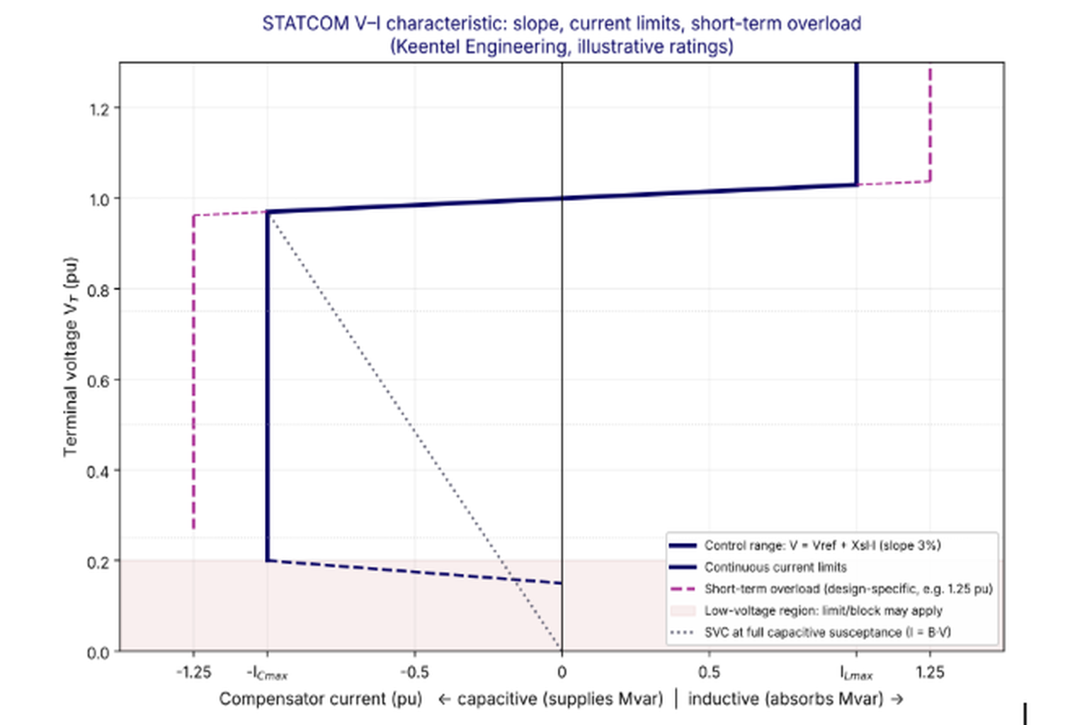
Figure 1. STATCOM V–I characteristic with a 3 percent slope, continuous current limits of 1.0 pu, an illustrative 1.25 pu short-term overload and a possible low-voltage limiting region. The dotted line shows an SVC at full capacitive susceptance for comparison.
Four regions are visible:
- The control range. Between the current limits, the device regulates voltage along a sloped line through the reference voltage. The slope means that the voltage it holds rises slightly as it absorbs reactive power and falls slightly as it supplies it.
- The continuous capacitive limit. Once the device reaches its maximum capacitive current, the characteristic becomes a vertical wall. Further voltage drop no longer increases current; the current stays at the limit, so reactive output falls in proportion to voltage.
- The continuous inductive limit. The mirror image on the right: at maximum inductive current the device can absorb no more, and further voltage rise is uncontrolled by the STATCOM.
- The short-term region and the low-voltage region. Many designs can exceed the continuous current for a limited time, shown by the dashed walls. At very low voltage, many converters reduce current or block entirely to protect the valves or because their synchronization cannot track a collapsed voltage.
Key terms used in this guide
| Term | Meaning in this guide |
|---|---|
| STATCOM | Static synchronous compensator: a shunt-connected voltage-source converter (VSC) that exchanges reactive current with the grid |
| SVC | Static var compensator: a shunt device built from thyristor-controlled reactors (TCR), thyristor-switched capacitors (TSC) and filters, acting as a variable susceptance |
| V–I characteristic | The steady-state relationship between terminal voltage and compensator current, including slope and limits |
| V–Q characteristic | The same relationship expressed in reactive power; for a STATCOM at its limit, Q falls in proportion to V |
| Reference voltage (Vref) | The voltage the regulator holds when the compensator current is zero |
| Slope (droop, Xsl) | The ratio of voltage change to compensator current change in the control range, in percent on the compensator rating |
| ICmax, ILmax | Maximum continuous capacitive and inductive currents |
| Short-term overload | Current above the continuous limit that the converter can carry for a stated time, limited by semiconductor junction temperature and other stresses |
| Minimum operating voltage | The voltage below which the converter limits, reduces or blocks its current |
| Coupling transformer | The transformer, or phase reactor, connecting the converter to the transmission bus; its reactance shapes the converter's voltage requirements |
| MMC | Modular multilevel converter: the dominant STATCOM topology for transmission ratings, built from many submodules in each arm |
| MSC, MSR, TSC | Mechanically switched capacitor, mechanically switched reactor and thyristor-switched capacitor, often coordinated with a STATCOM |
| Slow reset | A slow control that drifts the STATCOM's output back toward a target band by adjusting the reference or switching shunt banks, preserving dynamic reserve |
| Ssc, SCR | Short-circuit MVA at the bus and short-circuit ratio relative to a device or plant rating |
| FIDVR | Fault-induced delayed voltage recovery, caused mainly by stalled induction motor loads such as residential air conditioners |
| POI, RPA | Point of interconnection and reference point of applicability (the point where IEEE 2800 requirements are measured) |
| E-STATCOM | A STATCOM with an energy store, usually batteries or supercapacitors, that can also exchange real power |
Quick reference: the relationships that matter
| Relationship | Expression | What it tells you |
|---|---|---|
| Control-range characteristic | V = Vref + Xsl·I (inductive current positive) | Steady-state voltage held by the regulator for a given output |
| STATCOM at capacitive limit | Q = V·Imax | Output falls in proportion to voltage |
| SVC at capacitive limit | Q = B·V² | Output falls with the square of voltage |
| STATCOM-to-SVC output ratio at equal nameplate | 1/V | 1.11 at 0.9 pu, 1.43 at 0.7 pu, 2.0 at 0.5 pu |
| Voltage sensitivity of a bus | ΔV ≈ ΔQ/Ssc | Voltage authority of any reactive device, and the loop gain its regulator sees |
| Operating point with a Thevenin system | I = (Vth − Vref)/(Xs + Xsl) | How much of the range a given disturbance uses |
| Sharing between devices on one bus | Qi ∝ Si/Xsl,i | Larger ratings and smaller slopes take larger shares |
| Converter voltage behind the coupling reactance | Vc ≈ Vs ± Xt·I | Headroom needed for full capacitive and inductive current |
| Coupling transformer reactive loss | I²·Xt | Difference between converter-terminal and high-voltage-bus ratings |
| Current limit with real power | P² + Q² ≤ (V·Imax)² | How an E-STATCOM shares its current between real and reactive output |
Eight findings from Keentel's analysis
1. The STATCOM advantage is a current limit, not a magic constant. At its capacitive limit a STATCOM delivers Q = V·Imax while an SVC delivers Q = B·V². At 0.7 pu voltage a 150 Mvar STATCOM delivers 105 Mvar against 73.5 Mvar from a 150 Mvar SVC. At 0.9 pu the gap is only 11 percent. The advantage matters most exactly where FIDVR and voltage collapse begin.
2. Below a minimum voltage the advantage can vanish. Many converters limit or block below roughly 0.2 to 0.3 pu, depending on design. A characteristic that is drawn as a vertical line all the way to zero is a simplification.
3. The slope is a design decision, not a defect. A slope of 1 to 5 percent, most often 2 to 4 percent on transmission devices, keeps the device off its limits for small disturbances, makes reactive sharing between devices predictable and improves control stability on weak systems. With a zero slope and a 0.5 percent reference mismatch, two identical neighboring compensators can drive each other to opposite limits.
4. The operating point is set by the system as much as by the device. The compensator's sloped line intersects the system's Thevenin line. On a 40× short-circuit ratio bus with a 3 percent pre-disturbance voltage deficit, a 3 percent slope uses 55 percent of the capacitive range; a zero slope would hit the limit.
5. Short-term overload must be specified at the right terminals and for the right duration. In our thermal example, a 1.3 pu overload lasts about 2.2 seconds from light preload but under 1 second from full preload. "t < 1 s" is a possible design outcome, not a rule.
6. The coupling transformer consumes part of the rating. A STATCOM rated 150 Mvar at its low-voltage terminals behind a 12 percent transformer delivers about 132 Mvar capacitive at the high-voltage bus, and must produce 1.12 pu converter voltage to do so.
7. Hybrid designs stretch the budget. Combining a STATCOM with mechanically switched capacitors and a slow reset control restores dynamic range after the capacitors switch, at a fraction of the cost of a larger converter, but the capacitors' Q falls with V² during sags.
8. Models must carry the characteristic faithfully. Generic positive-sequence models represent slope, limits, overload and low-voltage logic only if their parameters are set to match the actual controls. Mismatches show up in MOD-033 validation and post-event analysis.
Engineering review of common claims
The table below reviews statements that commonly appear in short explanations of the STATCOM V–I characteristic and states the engineering position this guide supports.
| Common claim | Keentel engineering position |
|---|---|
| The STATCOM operates around a reference voltage of 1.0 pu | The reference is an adjustable setpoint, often between 0.95 and 1.05 pu, and is frequently moved by a slow outer control or the system operator. 1.0 pu is only an example. |
| The slight slope represents voltage regulation droop, allowing a small variation in voltage | Correct, but incomplete. The slope is deliberately chosen, typically 1 to 5 percent on the device rating, to share reactive power among devices, avoid hitting limits on small disturbances, coordinate with transformer tap changers and generator regulators, and keep the voltage loop stable as system strength changes. |
| When voltage falls, the STATCOM moves toward capacitive operation | Correct within the control range. The amount of current depends on the intersection of the slope with the system's Thevenin line, not on the voltage drop alone. |
| It maintains nearly constant capacitive current at significantly reduced voltage | True only between the device's minimum operating voltage and the current limit, and only if the converter, its synchronization and its protection are designed for it. Many designs limit or block below roughly 0.2 to 0.3 pu. Reactive power still falls in proportion to voltage. |
| This is a major advantage over the SVC | True during deep sags: at 0.5 pu the STATCOM delivers twice the Mvar of an equal-nameplate SVC. Near normal voltage the difference is small (11 percent at 0.9 pu), so equal nameplate is the wrong basis for comparison. |
| The STATCOM has maximum continuous capacitive and inductive current limits | Correct. The two limits need not be equal; asymmetric ratings are common, especially in hybrids where switched capacitors extend the capacitive range. |
| Beyond these limits it cannot provide additional continuous reactive current | Correct. |
| The transient rating applies for t < 1 s | Duration and magnitude are design-specific. Overload is limited by junction temperature, submodule capacitor voltage, cooling and protection. Some designs offer little or no capacitive overload; others offer 1.2 to 1.5 pu for one to several seconds. Overload duration also depends on preload. |
| The transient rating is symmetric on both sides | Not necessarily. Inductive overload at high voltage and capacitive overload at low voltage stress the converter differently. Capacitive overload may require higher converter voltage, which the modulation and submodule voltage limits may not allow. |
| The SVC has no comparable features | An SVC also has a slope, the same control-range behavior and, on the inductive side, a short-term TCR overload capability. Its capacitive limit is a fixed susceptance, so its current falls with voltage. |
The illustrative systems used in this guide
| System | Description | Used in |
|---|---|---|
| A | ±150 Mvar STATCOM at a 230 kV bus through a 34.5 kV coupling transformer of 12 percent reactance on 150 MVA | Worked Examples 1, 2, 3 and 8 |
| B | 230 kV load bus with 6,000 MVA short-circuit level under normal conditions and 3,500 MVA after a critical contingency | Worked Examples 3, 4 and 10 |
| C | Two compensators on a 345 kV network: a 200 Mvar and a 100 Mvar device | Worked Example 5 |
| D | ±100 Mvar STATCOM with two 50 Mvar mechanically switched capacitors at 138 kV | Worked Example 6 |
| E | 200 MW solar plant interconnecting at 230 kV with 34.5 kV collectors | Worked Example 11 |
| F | 138 kV load pocket with heavy residential air-conditioning load | Worked Example 9 |
All system data are illustrative. They are chosen to show the method and the size of the effects, not to represent any particular utility or project.
Part B — The STATCOM V–I Characteristic: An Engineering Guide
1. Why the characteristic deserves a deep look
Dynamic reactive power devices exist for one reason: voltage on a transmission network is a local quantity that depends on the balance of reactive power near the bus. Real power can travel long distances with modest voltage drop if the reactive power needed by the lines and loads is supplied close to where it is consumed. When generators retire, when lines are loaded harder, when large motor loads and inverter-based resources dominate a region, and when contingencies remove reactive sources or add reactive losses, voltage support has to come from somewhere else. Shunt capacitors are cheap but slow and their output collapses with the square of voltage. Synchronous condensers are robust and add inertia and short-circuit strength, but they are large rotating machines with significant losses and maintenance. Static var compensators were the workhorse of the late twentieth century. STATCOMs, based on the voltage-source converter, are now the default choice for many new dynamic reactive installations, both on transmission systems and inside inverter-based generating plants.
The V–I characteristic is where the device's design meets the system's needs. A planner's study assumes a characteristic; a supplier designs to a characteristic; a model represents a characteristic; a test verifies a characteristic. If those four versions disagree, the device will not perform during the event it was bought for. Three disagreements are especially common:
- Rating location. The planner assumed ±150 Mvar at the 230 kV bus; the supplier quoted ±150 Mvar at the converter's 34.5 kV terminals. The coupling transformer's reactive losses make the difference.
- Voltage range. The planner assumed full current down to 0.5 pu or lower; the supplier's design reduces current below 0.4 pu, or blocks below 0.2 pu during unbalanced faults.
- Overload. The planner counted on 1.3 pu current for two seconds during fault recovery; the supplier offered 1.3 pu for one second from no load, which shrinks to a fraction of a second from full load.
Each of these is visible on the V–I characteristic, if the characteristic is drawn completely and labeled at the right terminals. The rest of this guide is about drawing it completely.
2. Reading the characteristic: axes, conventions and per-unit bases
2.1 Axes and sign conventions
The classic textbook diagram puts terminal voltage on the vertical axis and compensator current on the horizontal axis, with capacitive current to the left and inductive current to the right. Three other conventions are common in practice, and confusion between them causes real errors:
| Convention | Where it appears | Capacitive (supplying) output shown as |
|---|---|---|
| Textbook V–I, capacitive left | FACTS textbooks, supplier brochures | Negative current, left of the axis |
| Generator convention, Q positive out | Power flow and stability programs, NERC data submittals | Positive Mvar |
| Load convention, susceptance positive | Some SVC controls and older specifications | Positive susceptance (capacitive B) |
| Inductive positive current | Some converter control documentation | Negative current |
A specification, a model and a test report should each state their convention explicitly. Keentel's practice is to state reactive output in generator convention (capacitive is positive Mvar out of the device) in study reports and model data, and to reproduce the supplier's convention only in control-setting tables, with a clear note.
2.2 Which voltage and which current
A STATCOM usually connects to the transmission bus through a coupling transformer, and the converter itself operates at a medium voltage, commonly 13.8 kV to 34.5 kV for transmission-scale units, or at 34.5 kV collector voltage inside renewable plants. There are therefore at least three places where voltage and current can be measured and rated:
- The converter terminals, where semiconductor current and converter voltage limits apply.
- The low-voltage side of the coupling transformer, which may coincide with the converter terminals or be separated by a phase reactor.
- The high-voltage bus or point of interconnection, where the planner's requirement applies and where the regulator usually measures voltage.
The current limit is physically a converter-terminal quantity. The planner's requirement is a high-voltage-bus quantity. The difference between them is the coupling transformer, which consumes reactive power proportional to the square of current and shifts the voltage the converter must produce. Worked Example 2 quantifies this.
2.3 Per-unit bases
The slope is quoted in percent on the compensator's own rating, usually its continuous capacitive or inductive Mvar rating at 1.0 pu voltage. A 3 percent slope on a 150 MVA base is a reactance of 0.03 pu on 150 MVA, which corresponds to a voltage change of 3 percent from zero to full current. On a 100 MVA system base, the same slope is 0.02 pu. Mixing bases is the single most common error in transferring slopes from specifications into planning models. A specification that says "slope adjustable 1 to 5 percent" must state its base.
2.4 The three regions in equations
Within the control range, using inductive current as positive:

At the capacitive limit the current is fixed and reactive output in generator convention is:

At the inductive limit:

Compare the SVC at its capacitive limit, where it is a fixed susceptance:

These four equations contain most of the practical comparison between the two technologies. The STATCOM's reactive output falls linearly with voltage at its limit; the SVC's falls with the square of voltage.
3. The physics behind the characteristic
3.1 The voltage-source converter as a controllable voltage behind a reactance
A STATCOM's converter synthesizes a three-phase AC voltage from a DC capacitor (in a two- or three-level converter) or from many submodule capacitors (in a modular multilevel converter). Viewed from the grid, it is a controllable voltage source Vc behind the coupling reactance X of the phase reactor and transformer. If the converter voltage is in phase with the system voltage Vs, no real power flows and the current is purely reactive:
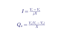
When Vc is greater than Vs, the converter supplies reactive power to the system (capacitive operation). When Vc is less than Vs, it absorbs reactive power (inductive operation). A small phase shift between Vc and Vs lets the converter draw just enough real power to cover its losses and hold its DC voltage, which is how the DC capacitor stays charged without an external source.
This simple picture explains why a STATCOM's current, not its susceptance, is limited. The semiconductor devices carry the full AC current. Their thermal and safe operating area limits translate directly into a maximum current magnitude, regardless of whether that current is capacitive or inductive and largely regardless of the system voltage.
3.2 Why the converter voltage matters for capacitive output
To supply capacitive current, the converter must produce a voltage higher than the system voltage by the drop across the coupling reactance. If the converter voltage is already near its maximum (set by the DC voltage, the number of submodules and the modulation index), then capacitive current is limited at high system voltage. To absorb inductive current, the converter voltage must be below the system voltage, which is usually easy, but very high system voltage still requires the converter to synthesize a waveform at or near the system peak voltage.
This creates a subtle feature of real characteristics: the capacitive current limit may itself be voltage-dependent at the top of the voltage range, and the inductive limit may be voltage-dependent at the bottom. The diagram in Figure 1 shows idealized vertical walls; the real walls can bend. Suppliers usually state a voltage range, for example 0.9 to 1.1 pu at the high-voltage bus, over which full rated current is available in both directions, and a wider range over which reduced current is available.
3.3 Converter topologies and what they imply for the characteristic
| Topology | Typical use | Implications for the V–I characteristic |
|---|---|---|
| Two- and three-level VSC with PWM | Smaller STATCOMs, distribution and plant-level units, many IBR plant STATCOMs | Higher switching frequency and losses; overload limited by device junction temperature; filters often needed |
| Multi-pulse or multi-level transformer-based | Early transmission STATCOMs | Complex transformers; largely superseded |
| Modular multilevel converter (MMC), chain-link cells | Most new transmission STATCOMs | Low harmonics, low switching losses, scalable; overload limited by device temperature and submodule capacitor voltage ripple; capacitive overload may need extra submodule voltage margin |
| Cascaded H-bridge, delta or star connected | Transmission and industrial units | Delta connection can circulate zero-sequence current to balance cells during unbalanced operation; affects unbalanced capability |
In an MMC or cascaded H-bridge STATCOM, the energy stored in submodule capacitors oscillates with each cycle. At higher current, the oscillation grows, and with it the peak submodule voltage. The capacitive overload limit can therefore be set by capacitor voltage rather than semiconductor temperature. This is one reason capacitive and inductive overloads are not necessarily equal.
3.4 How the controller enforces the characteristic
Inside the controller, the characteristic is enforced in the synchronous reference frame. The PLL aligns the d-axis with the measured positive-sequence voltage. In that frame, the d-axis current is in phase with voltage (real power) and the q-axis current is in quadrature (reactive power). The outer voltage regulator with slope produces a q-axis current reference; a small d-axis reference holds the DC or submodule energy. The current limiter then clips the references before the inner current loop acts:
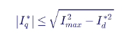
Because the d-axis current needed for losses is small, the q-axis limit is very close to Imax in a conventional STATCOM. In an E-STATCOM exchanging real power, the d-axis current can be large and the reactive limit shrinks accordingly.
Three practical consequences follow from this structure:
- The vertical walls in Figure 1 are current limits applied to a reference. When the voltage regulator asks for more than the limit, its integrator must be prevented from winding up, or the device will be slow to come off the limit when voltage recovers. Anti-windup design is a common source of differences between suppliers and between a device and its generic model.
- The limit can be changed dynamically. Thermal models can raise it briefly (short-term overload) or lower it (high temperature, loss of cooling redundancy, failed submodules). The characteristic in service is therefore the characteristic at that moment, and the controller should report its present capability to operators.
- During unbalanced faults, the frame changes. Controllers that inject negative-sequence current run a second, negative-sequence frame and allocate the phase current limit between frames. The simple V–I picture then describes only the positive-sequence part of the response.
Worked Example 1 — Converter-side current for a ±150 Mvar STATCOM
Problem. System A uses a ±150 Mvar STATCOM. Compare the converter-side current if the converter operates at 13.8 kV or at 34.5 kV, and find the current rating needed to deliver the full 150 Mvar at 0.9 pu voltage.
Solution. At rated voltage, current is the rated Mvar divided by √3 times line-to-line voltage:
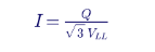
| Converter voltage | Current at 1.0 pu V for 150 Mvar | Current needed for 150 Mvar at 0.9 pu V | Ratio |
|---|---|---|---|
| 13.8 kV | 6,276 A | 6,973 A | 1.111 |
| 34.5 kV | 2,510 A | 2,789 A | 1.111 |
Interpretation. A 150 Mvar rating at 1.0 pu delivers only 135 Mvar at 0.9 pu. If the planning study needs 150 Mvar at 0.9 pu, the converter's current rating must be 11 percent higher, not its Mvar nameplate at 1.0 pu. The choice of converter voltage drives the current that the valves, bus work, breakers and transformer low-voltage windings must carry: at 13.8 kV the current exceeds 6,000 A, which is one reason transmission STATCOMs commonly use converter voltages in the 20 to 35 kV range or higher. Specifications should state the required Mvar at a stated voltage at a stated terminal, not a bare Mvar number.
Worked Example 2 — What the coupling transformer takes from the rating
Problem. In System A the converter connects to the 230 kV bus through a 150 MVA transformer with 12 percent reactance. The converter is rated 1.0 pu current. What converter voltage is needed for full capacitive and inductive current at several high-voltage-bus voltages, and how much reactive power reaches the 230 kV bus?
Solution. With purely reactive current and the transformer reactance Xt on the converter base, the converter voltage magnitude is approximately:

| HV bus voltage (pu) | Converter voltage, full capacitive (pu) | Converter voltage, full inductive (pu) |
|---|---|---|
| 0.95 | 1.07 | 0.83 |
| 1.00 | 1.12 | 0.88 |
| 1.05 | 1.17 | 0.93 |
| 1.10 | 1.22 | 0.98 |
Note how different the two factors are. An engineer who enters 0.70 into both fields of a relay that uses the separate format will under-compensate the resistive part by a factor of 1.7, which shifts the measured fault impedance and alters the resistive coverage near the reach point.
Step 4. Secondary conversion. With 2000:5 CTs (ratio 400) and 230 kV to 115 V VTs (ratio 2000), the secondary-to-primary factor is 400/2000 = 0.2:

To deliver 150 Mvar capacitive at the 230 kV bus at 1.0 pu voltage, the converter must produce about 168 Mvar, that is, 12 percent more.
Interpretation. The coupling transformer makes the characteristic asymmetric when it is viewed from the high-voltage bus: it subtracts from capacitive output and adds to inductive absorption. It also sets the converter voltage headroom. A converter asked to deliver full capacitive current while the 230 kV bus is already at 1.05 to 1.10 pu, for example in var or power factor control mode supporting a remote bus during heavy transfers, must produce 1.17 to 1.22 pu voltage and may hit its modulation limit; if the supplier did not design for that case, the capacitive limit will bend at high voltage. Conversely, low transformer reactance increases fault current contribution from the grid into the converter and the size of switching harmonics reaching the grid. Transformer reactance is therefore a joint design choice, and the rating point must be stated at the high-voltage bus.
How Keentel Engineering helps here: We translate planning requirements into terminal-specific ratings, accounting for the coupling transformer, auxiliary load, voltage range and per-unit bases, so that the supplier's quoted characteristic and the planner's assumed characteristic are the same characteristic. Our specification reviews flag ratings stated at the wrong terminals and slopes stated on the wrong base before contracts are signed.
4. The slope: why a voltage regulator should not regulate perfectly
4.1 Definition
The slope, also called droop or current compensation, is the deliberate tilt of the characteristic in the control range. With a slope Xsl in per unit on the compensator rating, the steady-state voltage the regulator holds is:
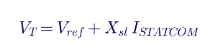
A slope of 3 percent means that the regulated voltage is 3 percent below the reference at full capacitive current and 3 percent above it at full inductive current. The total voltage span of the control range is therefore twice the slope, 6 percent for a 3 percent slope.
The slope is implemented in the controller, not in hardware. The regulator measures terminal voltage and compensator current (or reactive power), forms a corrected voltage error, and drives it to zero with an integral or proportional-integral regulator:

Because the regulator integrates this corrected error, steady state is reached on the sloped line rather than at exactly Vref. Some designs implement the slope on reactive power instead of current. At voltages near 1.0 pu the two are nearly equivalent; at depressed voltage they differ, and the model must use the same form as the actual controller.
4.2 Why a slope is used
A perfectly flat characteristic, with zero slope, would hold voltage exactly at the reference until the device reached its limit. That sounds ideal but has five practical drawbacks:
1. Uncontrolled sharing. Two devices with zero slope regulating nearby buses each try to hold their own reference exactly. Any small difference in reference, measurement error or transducer calibration makes them fight, one pushing capacitive and the other inductive, until one or both reach a limit. Worked Example 5 shows the effect.
2. Wasted range. With zero slope, the device swings to its limit for any disturbance that moves the system's Thevenin voltage by more than a small amount. It then has no reserve left for the next, larger disturbance. A slope makes the device's response proportional to the disturbance and keeps a reserve.
3. Interaction with slower controls. Transformer load tap changers, generator automatic voltage regulators and switched shunt controllers all respond to voltage. A flat-characteristic STATCOM holds the voltage those controls see at exactly the reference, so they never act, and the STATCOM absorbs the full steady-state burden. A slope lets voltage drift slightly, which lets slower devices take over, freeing the STATCOM's dynamic range for the next event.
4. Control stability. The voltage loop gain depends on system strength. A slope adds a proportional feedback path that reduces the effective loop gain and improves the stability margin when the grid weakens after contingencies.
5. Linear operation over a wider range. With a slope, the device's output in steady state is approximately proportional to the voltage deviation, which makes its behavior predictable and easier to coordinate with planning criteria.
The price of the slope is a small steady-state voltage error. On a strong bus that error is barely noticeable; on a weak bus the slope's effect is smaller relative to the system's own voltage sensitivity. Worked Example 3 makes this concrete.
4.3 Typical values
| Application | Typical slope (percent on compensator rating) | Comments |
|---|---|---|
| Transmission STATCOM or SVC regulating a strong bus | 2 to 4 | Most common range; 3 percent is a frequent default |
| Transmission device on a weak bus or radial system | 3 to 5 | Larger slope improves stability margin and limits sensitivity to Thevenin changes |
| Several devices sharing a region | 2 to 5, coordinated | Slopes chosen so that each device's share is proportional to its rating, or deliberately weighted |
| Plant-level STATCOM inside an IBR plant | Set by the plant controller design | The plant controller usually applies droop at the point of interconnection; the STATCOM may run in var or current control slaved to it |
| Industrial load compensation (flicker, arc furnaces) | 0 to 2, or reactive power control mode | Load compensation often regulates reactive power or flicker, not voltage |
These ranges are typical, not mandatory. The right slope comes from a coordination study, not a table.
4.4 The operating point: compensator slope meets system line
The bus voltage seen by the compensator depends on the network behind it. For small changes, the network can be represented by a Thevenin equivalent: an open-circuit voltage Vth (the voltage the bus would have with the compensator at zero output) behind a reactance Xs. On the compensator's base, with inductive current positive:

The steady-state operating point is where the system line meets the compensator's slope:

subject to the current limits. The STATCOM's output is the system's voltage deficit or surplus divided by the sum of the system and slope reactances.
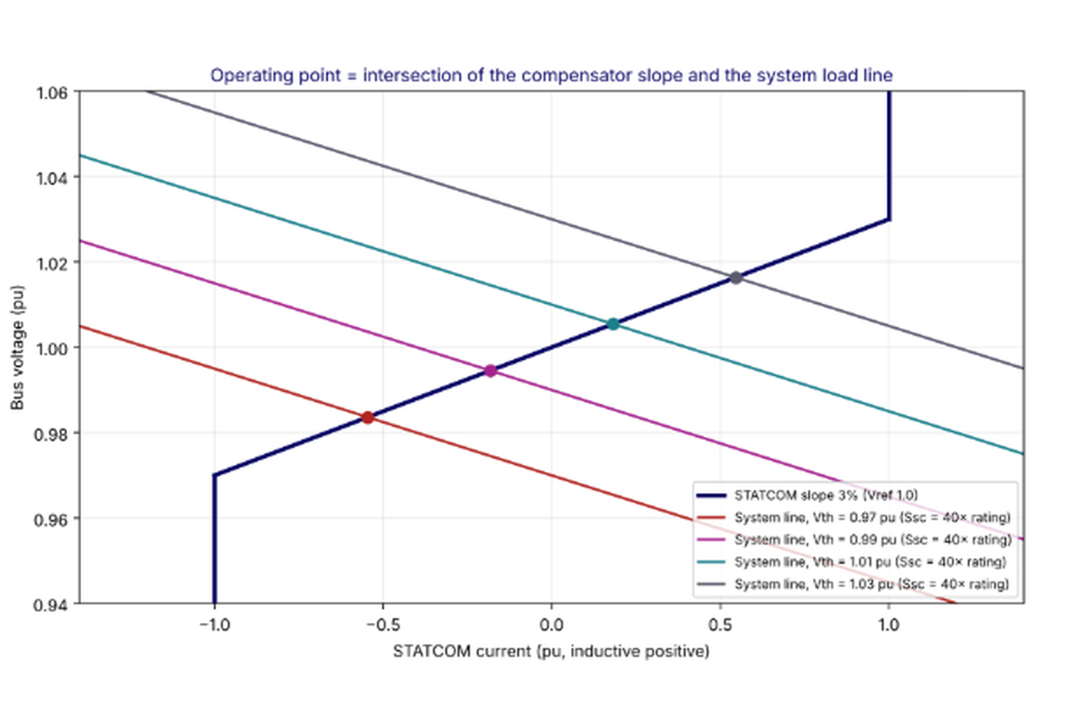
Figure 2. The steady-state operating point is the intersection of the compensator's sloped characteristic and the system's Thevenin line. As the system voltage moves, the intersection slides along the slope until it reaches a current limit.
Worked Example 3 — Where does a 3 percent slope put the operating point?
Problem. System A's ±150 Mvar STATCOM sits on a 230 kV bus with a short-circuit level of 6,000 MVA, forty times the device rating. The reference is 1.0 pu. Find the operating point for Thevenin voltages of 0.97, 0.99, 1.01 and 1.03 pu with slopes of 0, 1, 3 and 5 percent.
Solution. The system reactance on the 150 MVA base is Xs = 150/6,000 = 0.025 pu. Applying the intersection equation and clipping at ±1.0 pu current:
| Vth (pu) | Slope | Current (pu, capacitive negative) | Bus voltage (pu) | Output (Mvar, capacitive positive) |
|---|---|---|---|---|
| 0.97 | 0% | −1.20 → limited to −1.00 | 0.995 | +149 |
| 0.97 | 1% | −0.857 | 0.991 | +128 |
| 0.97 | 3% | −0.545 | 0.984 | +81 |
| 0.97 | 5% | −0.400 | 0.980 | +59 |
| 0.99 | 3% | −0.182 | 0.995 | +27 |
| 1.01 | 3% | +0.182 | 1.005 | −27 |
| 1.03 | 0% | +1.20 → limited to +1.00 | 1.005 | −151 |
| 1.03 | 3% | +0.545 | 1.016 | −83 |
Interpretation. With zero slope, a 3 percent Thevenin deficit drives the STATCOM to its full 150 Mvar capacitive limit and it still cannot quite hold 1.0 pu. Any further disturbance meets a device with no reserve. With a 3 percent slope, the same deficit uses about 55 percent of the range, holds the bus at 0.984 pu and leaves 70 Mvar of fast reserve for a fault or a second contingency. The cost is a 1.6 percent voltage difference compared with a flat characteristic. The comparison also shows why the choice is system-specific: on a weaker bus, Xs is larger, the slope's share of the total reactance is smaller and the voltage penalty of a slope is smaller still.
Worked Example 4 — How far does reactive power move voltage?
Problem. Estimate the voltage change caused by a 100 Mvar step at buses with short-circuit levels of 8,000, 5,000, 3,000 and 1,500 MVA.
Solution. For a predominantly reactive network, the voltage sensitivity is approximately:

| Short-circuit level (MVA) | ΔV for 100 Mvar |
|---|---|
| 8,000 | 1.25% |
| 5,000 | 2.00% |
| 3,000 | 3.33% |
| 1,500 | 6.67% |
Interpretation. The same device has five times more voltage authority on a 1,500 MVA bus than on an 8,000 MVA bus. The voltage loop's gain changes by the same factor, which is why a regulator tuned on the strong system can oscillate when lines trip and the bus weakens. It is also why a slope that is barely noticeable on a strong bus becomes a stabilizing element on a weak one. The approximation assumes a mostly reactive Thevenin impedance and modest angle changes; at buses with high resistance-to-reactance ratios, such as some 69 kV and 34.5 kV systems, real power flow also affects voltage and a full power-flow sensitivity should be used.
4.5 Reactive power sharing between compensators
When two or more dynamic devices regulate the same area, the slope determines how they share. For two devices regulating the same bus voltage, each device's output in the control range is proportional to its rating divided by its slope:

Equal sharing in proportion to ratings requires equal slopes on each device's own base. A deliberate preference, for example letting a newer STATCOM carry more of the steady-state load than an older SVC near the end of its life, is achieved by giving it a smaller slope.
Worked Example 5 — Sharing and fighting between two compensators
Problem. System C has two compensators electrically close on a 345 kV network: device A rated 200 Mvar with a 2 percent slope and device B rated 100 Mvar with a 4 percent slope. (a) How do they share when the regulated voltage falls 0.5, 1 and 2 percent below their common reference? (b) Device B's reference is 0.5 percent higher than A's because of a transducer calibration difference. How much reactive power circulates between them with slopes of 3, 1 and nearly 0 percent, if the area short-circuit level is 4,000 MVA?
Solution (a). Using the sharing equation:
| Voltage drop below Vref | Device A output (Mvar) | Device B output (Mvar) |
|---|---|---|
| 0.5% | 50 | 12.5 |
| 1.0% | 100 | 25 |
| 2.0% | 200 (limit) | 50 |
Device A carries four times the reactive power of device B for any voltage deviation, because it has twice the rating and half the slope. At a 2 percent deficit A is already at its limit while B is only half loaded, so B's reserve becomes the area's only fast reserve.
Solution (b). Solving the bus voltage and both outputs together with the 4,000 MVA system:
| Slopes (both devices) | Bus voltage (pu) | Device A (Mvar) | Device B (Mvar) | Circulating reactive power |
|---|---|---|---|---|
| 3% | 1.001 | −7.9 | +12.7 | about 8 Mvar |
| 1% | 1.001 | −29.4 | +35.3 | about 30 Mvar |
| ≈0% | 1.000 | −99.8 | +100 (limit) | about 100 Mvar, B at its limit |
Interpretation. With a 3 percent slope, a 0.5 percent reference mismatch costs only about 8 Mvar of circulating reactive power, which is negligible. With a nearly flat characteristic, the same mismatch drives B to its full capacitive limit and A to absorb almost the same amount: the devices fight, the area loses its dynamic reserve in both directions and losses rise. The case for slopes is therefore not mainly about voltage accuracy; it is about keeping multiple devices from wasting each other's range.
4.6 Coordination with tap changers, shunts and generators
The slope is one layer in a hierarchy of voltage controls:
| Layer | Typical time frame | Role |
|---|---|---|
| STATCOM or SVC fast voltage control | Tens of milliseconds | Hold voltage through faults, swings and sudden load changes |
| Generator AVRs and IBR plant controllers | Hundreds of milliseconds to seconds | Regulate plant terminal or POI voltage, share reactive load |
| STATCOM slow reset and switched shunt control | Seconds to minutes | Restore the STATCOM's dynamic reserve by moving steady-state reactive load to switched capacitors or reactors |
| Transformer load tap changers | Tens of seconds to minutes | Regulate distribution voltage, with intentional delays |
| Operator and automatic voltage schedules | Minutes to hours | Set references, switch shunts and schedule generator voltages under VAR-001 and VAR-002 |
Coordination principles that follow from this hierarchy:
- Separate time frames. Faster controls should finish their response before slower ones begin, and slower ones should not chase the faster ones' transients. Tap changer delays of 30 to 60 seconds and slow reset time constants of tens of seconds to minutes are typical.
- Leave room for slower controls to act. A slope or a deadband allows voltage to move enough for tap changers and shunt controllers to see a sustained deviation.
- Avoid opposing objectives. A tap changer raising distribution voltage after a contingency increases load and reactive demand; a STATCOM holding transmission voltage absorbs the consequence. The combined response must be studied over the full post-contingency time frame, not just the first few seconds.
- Coordinate references. A STATCOM reference set at 1.02 pu next to a generator scheduled at 1.00 pu creates a permanent tug of war; schedules should be set consistently.
4.7 Selecting the slope: a practical procedure
1. Define the regulated bus and the devices sharing it. Include generators, IBR plants, SVCs, STATCOMs and switched shunts within electrical reach.
2. Calculate Thevenin impedances at the regulated bus for the normal system and for the credible contingencies, using the planning model.
3. Choose a target share for each dynamic device in proportion to rating or by deliberate preference.
4. Check steady-state utilization. For the expected range of Thevenin voltages under normal and contingency conditions, the steady-state output should leave enough dynamic reserve for the design fault. A common target is to keep steady-state output below 25 to 50 percent of the rating, with switched shunts or slow reset doing the rest.
5. Check stability. Using a validated dynamic or EMT model, confirm that the voltage loop is stable and adequately damped across the full range of system strengths, including the weakest credible case.
6. Check interactions. Simulate the post-contingency period long enough for tap changers and shunt controllers to act, typically several minutes in quasi-steady-state or long-term dynamic simulation.
7. Document and model. Enter the final slope in the planning model in the model's own convention and base, and record it in the MOD-032 data submittal and the setting files.
4.8 Regulating a remote bus and line drop compensation
Most transmission STATCOMs regulate the voltage of the bus they connect to. Sometimes the voltage that matters is elsewhere: a load bus at the end of a radial 115 kV line, or the point of interconnection of a plant whose STATCOM sits at the collector substation. Two approaches are used.
- Remote voltage measurement. The regulator uses a voltage measured at the remote bus, transmitted over a communication link. This regulates the right quantity but adds latency and a dependence on communications. Control logic must define a fallback, usually reverting to local regulation, if the link fails.
- Line drop compensation. The regulator estimates the remote voltage from the local voltage and the measured current through the intervening line or transformer impedance. It is simple and needs no communications, but its accuracy depends on knowing the impedance and on the remote bus being radially fed. In a meshed network, other flows into the remote bus make the estimate wrong.
The choice changes the effective slope at each bus. A device that regulates its own bus with slope Xsl, seen from a remote bus reached through a line of reactance Xline (on the same base), behaves as if its slope were Xsl + Xline, because the line's own voltage drop adds to the slope; the remote bus gets weaker regulation than the setting suggests. Line drop compensation removes that line reactance from the remote characteristic, but it also reduces the slope seen at the device's own bus to Xsl − Xcomp, where Xcomp is the compensation reactance. If Xcomp is larger than Xsl, the characteristic at the local bus has a negative slope, which is destabilizing when other devices regulate nearby. Coordination studies for remote regulation should therefore compute the effective slope at every bus that matters, not just read the setting in the controller.
Plant-level STATCOMs in IBR plants face this question routinely: the power plant controller regulates the POI, which may be several miles and one or two transformers away from the STATCOM. The plant's droop is then defined at the POI by the plant controller, and the STATCOM's own local control acts mainly as a fast inner loop.
How Keentel Engineering helps here: We select and coordinate slopes, deadbands and references for STATCOMs, SVCs, IBR plant controllers and switched shunts using Thevenin analysis, Q–V curves and dynamic simulation across normal and contingency conditions. Our reports show how each device shares reactive power, how much dynamic reserve remains after each design event and how the fast and slow controls coordinate, so that operators and planners can trust the settings.
5. Control modes and the control hierarchy inside the STATCOM
5.1 The control structure
A modern STATCOM controller is layered. From the inside out:
- Valve and submodule control. Firing pulses, submodule capacitor voltage balancing, and protection against overcurrent and overvoltage at the device level. Time scale: microseconds.
- Inner current control. Usually in a synchronous reference frame (dq) aligned with the grid voltage by a phase-locked loop (PLL). The q-axis current is the reactive current; the d-axis current covers losses and regulates the DC or submodule energy. In an MMC, additional loops control circulating current. Time scale: about a millisecond.
- Outer control. The voltage regulator with slope, or a reactive power, power factor or current controller, which produces the reactive current reference. Time scale: tens of milliseconds.
- Supervisory and slow controls. Slow reset, switched shunt coordination, gain supervision, power oscillation damping, operator interfaces and protective limiters. Time scale: seconds to minutes.
The V–I characteristic is the steady-state picture of the outer control and the current limiter. Dynamic behavior, including overshoot, settling and interaction with the grid, comes from the inner and outer loops together.
5.2 Outer control modes
| Mode | What it regulates | Typical use | Effect on the characteristic |
|---|---|---|---|
| Voltage control with slope | Bus voltage | Transmission voltage support, the default for utility STATCOMs | Sloped line through Vref, current limits at the ends |
| Voltage control with deadband | Bus voltage outside a band | Avoids continuous small-signal activity; leaves steady-state regulation to slower devices | Flat segment at zero current within the band, sloped segments outside |
| Reactive power (var) control | A fixed Mvar output | Commissioning, special operating conditions, plant-level units slaved to a plant controller | Vertical line at the ordered current, until a voltage limiter overrides |
| Power factor control | Reactive power in proportion to a measured real power flow | Some IBR plants and industrial facilities | Output follows real power; voltage is not regulated directly |
| Current or susceptance reference | An external current order | Plant-level STATCOMs controlled by a power plant controller | The plant controller provides the slope at the POI |
| Undervoltage and overvoltage strategies | Special responses during faults | Fault ride-through, recovery support | Overrides normal control at abnormal voltages |
5.3 Deadband versus slope
A deadband is a voltage band around the reference within which the regulator does nothing. It is useful when a STATCOM should act only for dynamic events and leave steady-state regulation to switched shunts, tap changers and generators. It is not a substitute for slope: outside the deadband the device still needs a slope to share and to stay stable. A deadband also creates a discontinuity that can cause limit cycling with other controllers if it is too narrow. Deadbands of ±0.5 to ±2 percent are typical where they are used.
5.4 Slow reset: protecting dynamic reserve
The most important supervisory function in many transmission STATCOMs is slow reset, sometimes called slow susceptance regulation in SVCs. It slowly drives the STATCOM's steady-state output toward a target band near zero, either by adjusting the reference voltage within limits or by switching external shunt capacitors and reactors. The aim is to keep the fast converter range available for disturbances rather than tying it up in steady-state voltage support.
A typical slow reset logic:
- Monitor the STATCOM's steady-state output with a long filter, seconds to tens of seconds.
- If output stays above a capacitive threshold (for example 40 percent of rating) for longer than a delay, switch in a mechanically switched capacitor, or ramp the reference down by a small amount within an allowed band.
- If output stays below an inductive threshold, switch out a capacitor, switch in a reactor, or ramp the reference up.
- Respect minimum on and off times for mechanically switched banks so that capacitors can discharge and breakers are not overworked.
- Block slow reset during disturbances so that it does not undo the fast response while voltage is recovering
Worked Example 6 — A hybrid STATCOM with switched capacitors
Problem. System D is a ±100 Mvar STATCOM at 138 kV with two 50 Mvar mechanically switched capacitors (MSCs) under slow reset control. During a heavy load period, the STATCOM settles at 60 Mvar capacitive. Show how slow reset restores dynamic reserve, and compare the capacitive support available at 1.0, 0.9 and 0.7 pu voltage with one or both MSCs in service.
Solution. When the STATCOM output exceeds a 40 percent threshold for the set delay, slow reset closes the first MSC. The capacitor supplies about 50 Mvar at 1.0 pu voltage, so the STATCOM's output falls from about 60 Mvar to about 10 Mvar while the bus voltage stays nearly unchanged. Its fast capacitive reserve rises from 40 Mvar to about 90 Mvar.
Capacitive support during a voltage sag (the STATCOM at its current limit, the MSCs as fixed susceptances):
| Bus voltage (pu) | STATCOM at limit (Mvar) | One MSC (Mvar) | Two MSCs (Mvar) | STATCOM + two MSCs (Mvar) |
|---|---|---|---|---|
| 1.0 | 100 | 50 | 100 | 200 |
| 0.9 | 90 | 40.5 | 81 | 171 |
| 0.7 | 70 | 24.5 | 49 | 119 |
Interpretation. Slow reset converts a device that was 60 percent committed into one that is only 10 percent committed, more than doubling its fast reserve, using equipment that costs a fraction of extra converter capacity. During a sag the MSCs still help, but their contribution falls with the square of voltage, so at 0.7 pu two 50 Mvar capacitors provide less than the 100 Mvar STATCOM alone. The STATCOM is the part that holds up during deep sags; the MSCs do the steady-state work. A good hybrid design also checks the voltage step when each MSC switches (about 50/Ssc, roughly 1 to 2 percent on a typical 138 kV bus), the capacitor inrush and back-to-back switching duty, and the temporary overvoltage risk if the STATCOM trips while both MSCs are in service.
5.5 Gain supervision and adaptive control
Because the voltage loop gain scales with the inverse of short-circuit level, a regulator tuned for the intact system can become oscillatory when the system weakens. Common protective measures:
- Gain supervision. Detect sustained oscillation in the regulator output or the bus voltage and reduce gain in steps until it stops, then slowly restore.
- Adaptive gain. Estimate system strength online, for example from the voltage response to small output changes, and schedule gain accordingly.
- Conservative fixed tuning for the weakest credible system, accepting a slower response on the strong system.
Each approach has trade-offs. Gain supervision is reactive rather than preventive; adaptive gain requires reliable estimation; conservative tuning sacrifices speed. Specifications should require stable, well-damped response over the full range of credible system strengths and should require the supplier to demonstrate it on a real-time simulator model of the actual network.
5.6 Power oscillation damping
A STATCOM can modulate its reactive output to damp electromechanical oscillations, using a supplementary signal such as line power flow, bus frequency or angle difference. Damping effectiveness depends on the STATCOM's location relative to the oscillation mode shape and on the voltage sensitivity of the loads and lines nearby. A power oscillation damping (POD) function moves the operating point along and around the slope, so it consumes part of the dynamic range. Its output should be limited so that damping never takes the reserve needed for fault recovery.
5.7 Fault and recovery strategies
During a fault the measured voltage collapses and the regulator would normally drive the STATCOM to its capacitive limit. What happens next depends on the controller's fault strategy:
- Hold capacitive current during the fault. This supports the voltage at nearby buses and helps protection see the fault correctly, but it may contribute to overvoltage when the fault clears.
- Freeze or limit the output during the fault, then release it on recovery. This avoids overshoot but provides less support.
- Inject negative-sequence current during unbalanced faults, in addition to positive-sequence current, to reduce the negative-sequence voltage. Some IBR-related requirements now address negative-sequence current; transmission STATCOM specifications should state the expectation explicitly.
- Transition quickly to inductive operation when the fault clears and voltage overshoots, especially where capacitor banks, filters or long lines create temporary overvoltages.
The strategy should match the system's needs, be represented in the models used for planning and be verified during factory testing on a real-time simulator.
How Keentel Engineering helps here: We review control philosophies, specify control modes and slow reset logic, and verify regulator tuning across the full range of system strengths with positive-sequence and EMT simulation. For hybrid installations we design the switching logic for capacitors and reactors, check voltage steps, inrush and back-to-back switching duty, and make sure the slow controls protect the fast reserve instead of consuming it.
6. Continuous current limits
6.1 What sets the limit
The continuous current rating of a STATCOM is set by the thermal capability of the valves and their cooling system, the current rating of the phase reactors and coupling transformer, the bus work and switchgear at the converter voltage, and, in MMC designs, the submodule capacitor voltage ripple at full current. In practice the valve and cooling design dominates, and the rating is usually stated at a maximum ambient temperature.
Several practical consequences follow:
- Ambient derating. Air-cooled components and heat exchangers lose capability at high ambient temperatures. A rating stated at 40 °C may be lower at 46 °C in a Southwestern desert site, and higher in winter. Specifications should state the ambient range over which the rating must hold, using site design temperatures.
- Altitude. Air insulation and cooling are affected above about 1,000 meters (3,300 feet). Sites in the Mountain West may require derating or design adjustment.
- Redundancy. Many MMC designs include redundant submodules so that a failed cell can be bypassed without losing rating. Without redundancy, a single failure can force a reduced rating or a trip.
- Auxiliary power. Cooling pumps, fans, control power and building loads consume real power and sometimes reactive power. The net output at the high-voltage bus must account for them.
6.2 Symmetric and asymmetric ratings
STATCOMs are often specified symmetric, for example ±150 Mvar, but the system need is rarely symmetric. Voltage support after faults and contingencies requires capacitive range; absorbing reactive power during light load, after load rejection or with lightly loaded cables and long lines requires inductive range. Because a voltage-source converter's capability is fundamentally a current limit, a symmetric rating is natural for the converter. Asymmetric total ratings are achieved by adding fixed or switched capacitors (shifting the range toward capacitive) or reactors (shifting toward inductive). For example, a ±100 Mvar converter with a 50 Mvar fixed capacitor gives roughly +150/−50 Mvar at 1.0 pu, but the capacitor's share falls with V² during sags and its presence raises temporary overvoltage risk if the converter trips.
6.3 Current limit priority in E-STATCOMs
When a STATCOM has energy storage and can also exchange real power, the current limit must be shared between active and reactive current. The total current magnitude is limited:

The controller must decide which has priority. For voltage support during faults, reactive priority is usual. For fast frequency response after a generation loss, active priority may be preferred. The choice changes the characteristic: with active current flowing, the reactive current available at the limit is smaller. The priority setting should be specified, modeled and coordinated with any market or ancillary service obligations.
6.4 Positive- and negative-sequence current during unbalanced events
Most transmission faults are unbalanced. During a single-line-to-ground fault, the positive-sequence voltage may only drop to 0.6 to 0.7 pu while one phase collapses. If the STATCOM injects only positive-sequence current, the phase currents remain balanced and within the limit. If it also injects negative-sequence current to counter the voltage unbalance, the phase currents become unbalanced and the most heavily loaded phase reaches the limit first. The available positive-sequence current then has to be reduced:

as a conservative worst-case bound when the sequence currents align in the worst phase. Controllers therefore use limiting strategies that allocate the available phase current between sequences. Delta-connected cascaded converters must also manage cell energy balance during unbalanced operation, which may further limit negative-sequence capability. These details matter for protection, especially distance and negative-sequence directional elements on nearby lines, and should be represented in EMT studies.
How Keentel Engineering helps here: We specify continuous ratings at the right terminals and ambient conditions, check auxiliary load, derating and redundancy assumptions, and define current priority rules for E-STATCOMs and hybrid plants. For protection-sensitive locations, we evaluate the device's positive- and negative-sequence fault behavior with EMT models and confirm that nearby line relays still operate correctly.
7. Short-term overload ratings
7.1 What the dashed walls really mean
Diagrams of the STATCOM characteristic often show a second pair of walls beyond the continuous limits, labeled "transient rating", sometimes with a duration such as "t < 1 s". The idea is sound: semiconductors have thermal mass, so they can carry more than their continuous current for a short time before their junctions reach the maximum allowed temperature. But the magnitude and duration of that capability are not universal properties of STATCOMs. They are outcomes of a specific design, and they depend on:
- Semiconductor selection and margin. A supplier can choose devices with more or less current margin relative to the continuous rating. More margin costs money and increases losses slightly.
- Cooling design. Water-cooled valves with large heat exchangers recover faster than air-cooled ones; the coolant temperature at the start of the event matters.
- Preload. A converter operating near full output before the event has less thermal headroom than one operating near zero.
- Submodule capacitor voltage. In MMC designs, higher current increases capacitor voltage ripple. Capacitive overload may be limited by capacitor voltage rather than temperature.
- Converter voltage headroom. Capacitive overload requires a higher converter voltage, as Worked Example 2 showed. If the modulation is already near its limit, overload current may not be achievable at high system voltage.
- Protection settings. Valve overcurrent protection, transformer and reactor overload protection and control limiters must be coordinated with the intended overload, or the protection will act first.
- Transformer and reactor capability. These usually have more short-term thermal capacity than semiconductors, but their saturation and overvoltage limits can restrict inductive overload at high voltage.
The industry experience behind these points is consistent: some STATCOMs offer little or no capacitive overload; others are designed for overloads in the range of about 1.2 to 1.5 pu for durations from a fraction of a second to a few seconds; and inductive and capacitive overloads are often different. Any number used in a study must come from the supplier's guaranteed data for the specific design.
7.2 A simple thermal model
The junction temperature rise of a semiconductor is approximately proportional to its losses, which in turn grow roughly with the square of current. A first-order thermal model with an equivalent time constant τ is a useful planning approximation. If the steady-state temperature rise is proportional to I², and the device's maximum allowed temperature corresponds to a steady-state current Ith slightly above the continuous rating (the design margin), then from a preload current I0, an overload current Io can be held for:
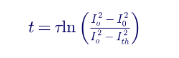
Real valves have several thermal time constants (junction to case, case to heat sink, heat sink to coolant), and suppliers use detailed multi-node models. The first-order model is not a design tool, but it shows the shape of the trade-offs.
Worked Example 7 — How long can a 1.3 pu overload last?
Problem. A STATCOM has an equivalent thermal time constant of 1.5 seconds and a design margin equivalent to a steady-state limit of 1.15 pu current (both illustrative). How long can it carry overloads of 1.2, 1.3 and 1.5 pu, starting from preloads of 0, 0.3, 0.6 and 1.0 pu?
Solution. Applying the first-order model:
| Preload (pu) | 1.2 pu overload (s) | 1.3 pu overload (s) | 1.5 pu overload (s) |
|---|---|---|---|
| 0.0 | 3.76 | 2.29 | 1.33 |
| 0.3 | 3.66 | 2.21 | 1.27 |
| 0.6 | 3.33 | 1.93 | 1.07 |
| 1.0 | 1.98 | 0.94 | 0.45 |
Interpretation. The same converter can sustain a 1.3 pu overload for more than two seconds from light preload but for less than one second from full preload. The preload sensitivity is the key lesson: a STATCOM that is already heavily loaded in steady state, because slow reset is missing or the system is short of steady-state reactive support, has less transient capability exactly when it is needed. A "t < 1 s" label on a diagram might describe the full-preload case of one design and the no-preload case of another. The specification and the planning model should therefore state overload capability as a function of preload, or at minimum for the worst preload expected during the design event. Re-arming time also matters: after an overload, the converter needs time to cool before a second overload is available, which affects performance during reclosing onto a fault or repeated events.
7.3 Capacitive versus inductive overload
| Aspect | Capacitive overload (low voltage) | Inductive overload (high voltage) |
|---|---|---|
| When needed | Fault recovery, voltage collapse, FIDVR, large motor starting | Temporary overvoltage after load rejection, fault clearing with capacitors connected, line energization, light load |
| Converter voltage required | Higher than system voltage; may hit modulation limits at high system voltage | Lower than system voltage; generally easier, but valve voltage stress increases with system voltage |
| MMC submodule stress | Higher capacitor voltage ripple at high current | Higher capacitor voltage ripple and higher valve voltage at high system voltage |
| Transformer and reactor | Thermal limit only | Thermal limit plus possible saturation at high voltage |
| Typical value in specifications | Varies widely; sometimes none | Often specified for TOV control; varies |
7.4 How SVCs compare
An SVC's capacitive limit is a fixed susceptance with no overload in the usual sense, because the capacitors are always fully connected at that point. Its inductive side, the thyristor-controlled reactor, can often carry short-term overload current at high voltage, and many SVC specifications include a TOV-related inductive overload rating. The comparison in short claims, that "the STATCOM has transient ratings and the SVC does not", is therefore not quite right: both technologies can have short-term ratings, and both must be specified explicitly.
7.5 Specifying short-term capability
A useful specification states short-term capability as a table rather than a single number:
| Item | Example specification wording (illustrative) |
|---|---|
| Continuous rating | ±150 Mvar at the 230 kV bus at 1.0 pu voltage, over the full site ambient range |
| Voltage range for continuous rated current | 0.90 to 1.10 pu at the 230 kV bus |
| Capacitive short-term current | 1.25 pu current for 2.0 s from a preload of 0.5 pu capacitive, at bus voltages from 0.5 to 1.0 pu |
| Inductive short-term current | 1.25 pu current for 1.0 s at bus voltages up to 1.30 pu |
| Re-arming | Short-term capability available again after 60 s at no more than 0.5 pu preload |
| Minimum operating voltage | Rated current maintained down to 0.3 pu positive-sequence voltage, with defined behavior below |
| Model and test requirements | Overload logic represented in the positive-sequence and EMT models; verified in factory testing |
The numbers above are examples only. The right values come from planning and EMT studies of the specific system and from the supplier's design.
How Keentel Engineering helps here: We determine how much short-term capability the system actually needs, from transient stability and EMT studies of the design events, and translate it into specification tables that state magnitude, duration, preload, voltage range and re-arming time. During bid evaluation we compare suppliers' guaranteed overload data on the same basis, and we make sure the overload logic is represented in the models the planner and the reliability coordinator will use.
8. Low-voltage performance: the STATCOM's real advantage
8.1 Linear versus quadratic
At its capacitive limit a STATCOM is a current source; an SVC is a fixed capacitor. The consequence is the most cited difference between the two technologies:

for devices with equal nameplate at 1.0 pu voltage.
Worked Example 8 — Capacitive output of ±150 Mvar devices during sags
Problem. Compare the capacitive output of a ±150 Mvar STATCOM at its current limit and a ±150 Mvar SVC at full capacitive susceptance as voltage falls, and compute the SVC rating needed to match the STATCOM at each voltage.
Solution.

| Bus voltage (pu) | STATCOM (Mvar) | SVC (Mvar) | STATCOM ÷ SVC | SVC rating needed to match |
|---|---|---|---|---|
| 1.05 | 157.5 | 165.4 | 0.95 | 143 Mvar |
| 1.00 | 150.0 | 150.0 | 1.00 | 150 Mvar |
| 0.90 | 135.0 | 121.5 | 1.11 | 167 Mvar |
| 0.80 | 120.0 | 96.0 | 1.25 | 188 Mvar |
| 0.70 | 105.0 | 73.5 | 1.43 | 214 Mvar |
| 0.50 | 75.0 | 37.5 | 2.00 | 300 Mvar |
| 0.30 | 45.0 | 13.5 | 3.33 | 500 Mvar |
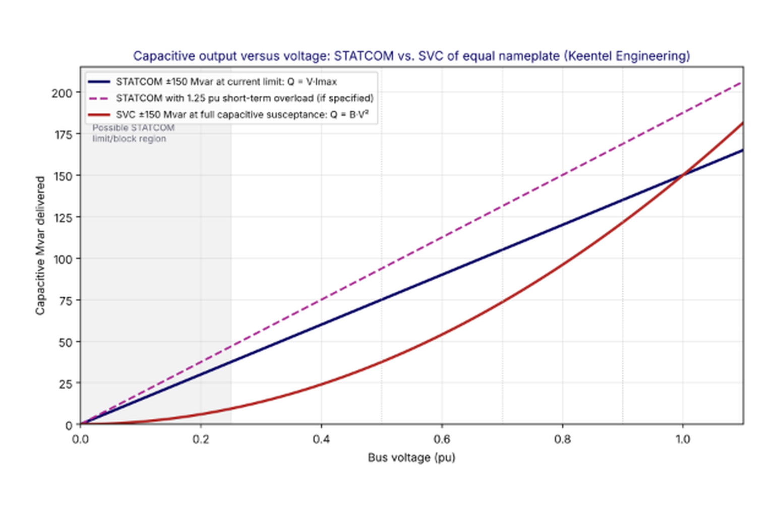
Figure 3. Capacitive output versus voltage for a STATCOM and an SVC with the same nameplate rating, and for the STATCOM with a 1.25 pu short-term overload. The shaded region marks voltages where some STATCOM designs limit or block.
Interpretation. Above 1.0 pu the SVC actually delivers slightly more than the STATCOM. Between 0.9 and 1.0 pu, where most steady-state planning criteria operate, the two are within 11 percent. The STATCOM's advantage becomes decisive below about 0.8 pu, which is where post-fault recovery, motor stalling and voltage collapse take place. The 0.3 pu row assumes the STATCOM maintains full current at that voltage, which must be confirmed for the specific design; if the converter blocks at 0.3 pu, its output there is zero.
8.2 The minimum operating voltage
Real STATCOMs do not keep full current down to zero voltage. Four mechanisms set a minimum:
- Synchronization. The PLL needs a measurable voltage to track phase angle. At very low positive-sequence voltage, or during severe unbalance and distortion, the PLL may lose accuracy. Designs differ in how they handle this: some freeze the angle, some switch to a different synchronization method, some block.
- Converter current control. Holding current at very low terminal voltage means the converter voltage is also very low, at the bottom of its modulation range, where control accuracy and harmonic performance can suffer.
- DC energy balance. The converter must draw a small amount of real power to cover losses and keep its DC or submodule capacitors charged. At very low voltage, the real current needed for that may compete with the reactive current.
- Protection. Valve protection may block the converter if current or capacitor voltage excursions during the fault exceed thresholds, especially at fault inception and clearing.
The resulting characteristic often looks like the dashed tail in Figure 1: full current down to a threshold, often specified somewhere around 0.2 to 0.4 pu, then reduced current, then possible blocking. Planners should obtain the actual characteristic, including thresholds, delays and recovery behavior after blocking, and make sure the model represents it. A STATCOM that blocks for 100 milliseconds after a deep fault and then ramps back slowly provides much less recovery support than one that stays online throughout.
8.3 Fault ride-through and recovery
A transmission STATCOM must ride through nearby faults and be ready to support recovery when they clear. Key aspects:
- Ride-through. The device should remain connected through faults cleared by normal and backup protection, including delayed clearing. For STATCOMs inside IBR plants, NERC PRC-029-1 and IEEE 2800 ride-through requirements apply at the plant level, and the STATCOM must not be the weak link.
- Current during the fault. Whether to hold full capacitive current, limit it or inject negative-sequence current, as discussed in Section 5.7.
- Recovery ramp. After clearing, the device should move smoothly from the fault response to normal regulation. Overshoot into inductive operation is often needed to limit TOV; sluggish recovery wastes support.
- Reclosing. If a line recloses onto a permanent fault, the STATCOM sees a second fault within about half a second to a few seconds. Thermal re-arming and protection logic must allow a second response.
8.4 Fault-induced delayed voltage recovery
FIDVR occurs when a fault depresses voltage long enough to stall single-phase residential air-conditioner compressors. Stalled motors draw several times their running current at a very low power factor, holding voltage down for several seconds until their thermal protection trips them, after which voltage can overshoot as load disappears and capacitors remain connected. Dynamic reactive devices help by supplying reactive power during the depressed-voltage period, raising voltage enough to allow some motors to reaccelerate and shortening the recovery.
Worked Example 9 — STATCOM versus SVC during FIDVR
Problem. System F is a 138 kV load pocket represented by a Thevenin source of 1.0 pu behind 0.05 pu reactance on 100 MVA (a 2,000 MVA short-circuit level). After a fault clears, the stalled motor load behaves as a constant impedance drawing 300 MW and 600 Mvar at 1.0 pu voltage. Compare the recovered bus voltage with no compensation and with STATCOMs or SVCs of 100, 200 and 300 Mvar, and find the rating needed to bring the bus up to 0.90 pu.
Solution. Solving the network iteratively, with the STATCOM as a current source at its limit and the SVC as a fixed susceptance:
| Device rating (Mvar) | Bus voltage with STATCOM (pu) | Bus voltage with SVC (pu) | STATCOM output (Mvar) | SVC output (Mvar) |
|---|---|---|---|---|
| None | 0.764 | 0.764 | 0 | 0 |
| 100 | 0.802 | 0.794 | 80 | 63 |
| 200 | 0.840 | 0.827 | 168 | 137 |
| 300 | 0.878 | 0.862 | 263 | 223 |
Ratings needed to reach 0.90 pu: about 358 Mvar of STATCOM or about 398 Mvar of SVC.
Interpretation. With stalled motors holding voltage near 0.76 pu, the STATCOM delivers 15 to 25 percent more reactive power than an SVC of the same rating, and the difference translates into roughly 40 Mvar less nameplate to reach the same recovery voltage. But the example also shows the limits of any shunt compensator against heavy stalled-motor load: hundreds of Mvar are needed to move voltage a few percent when the load itself absorbs 600 Mvar. Effective FIDVR mitigation usually combines dynamic reactive support with faster fault clearing, load-side measures such as compressor undervoltage protection, and in some areas under-voltage load shedding. Real FIDVR studies use composite load models with motor stalling and thermal tripping, as discussed in Section 10.
8.5 Post-fault overshoot: the other half of recovery
The moments after fault clearing are where the low-voltage and high-voltage sides of the characteristic meet. During the fault, the STATCOM was at or near its capacitive limit. When the breaker opens, voltage jumps back, often within a cycle. If the STATCOM is still producing full capacitive current, and if switched capacitors, filters and line charging are also in service, the bus voltage can overshoot well above 1.0 pu for several cycles. Motor loads that stalled during the fault are now reaccelerating and drawing heavy reactive current, so the overshoot may be followed by a second sag. The STATCOM must therefore move quickly from full capacitive output through zero to inductive output and back again.
Three characteristic-related details determine how well it does this:
- Anti-windup and limit exit. If the voltage regulator's integrator wound up during the fault, the STATCOM will remain capacitive for longer than it should after clearing, worsening the overshoot.
- Rate limits. Some controllers limit the rate of change of the current reference to protect the converter or avoid exciting resonances. A rate limit that is too slow turns a fast device into a slow one during recovery.
- Inductive capability at elevated voltage. The device needs its full inductive current at the overshoot voltage, which is exactly the high-voltage capability discussed in Section 9.
Planners should look at the full recovery waveform in time-domain studies, not only the minimum voltage during the fault. Many regional transient voltage criteria include both undervoltage and overvoltage limits after clearing, and a compensator that solves one can aggravate the other if its recovery logic is poorly tuned.
How Keentel Engineering helps here: We model low-voltage behavior faithfully, including minimum operating voltage, blocking and recovery logic, and use composite load models to evaluate FIDVR and post-fault recovery against TPL-001 and regional transient voltage criteria. Our studies show clients how much dynamic support is needed, where, and whether a STATCOM, an SVC, a synchronous condenser or a combination is the most economical way to meet the criteria.
9. The inductive side: high voltage and temporary overvoltage
9.1 Why the right half of the characteristic matters
Discussions of STATCOMs focus on the capacitive side because voltage collapse is dramatic. The inductive side is just as important in modern networks. Long 345 kV and 500 kV lines generate large amounts of charging reactive power at light load. Underground cables at 69 kV through 345 kV generate even more per mile. Large shunt capacitor banks and harmonic filters remain connected when load is lost. Inverter-based resources may stop absorbing reactive power when they trip. In each case, voltage can rise quickly, and a dynamic device that can absorb reactive power within a cycle or two keeps equipment within its temporary overvoltage (TOV) capability.
Typical events that call on the inductive side:
| Event | Mechanism | Time scale |
|---|---|---|
| Fault clearing with capacitors connected | Voltage recovers while capacitors and the STATCOM's own capacitive output are still high | First few cycles after clearing |
| Load rejection | Loss of large load or a tie line leaves line charging and capacitors uncompensated | Cycles to seconds |
| Line or cable energization | Charging current and the Ferranti effect raise the receiving-end voltage | Cycles to steady state |
| Light-load periods | Night-time charging surplus on lightly loaded EHV lines and cables | Hours |
| IBR plant trip | Loss of a plant that was absorbing reactive power | Cycles to seconds |
| Islanding of a load or generation pocket | Combination of the above with frequency excursions | Cycles to seconds |
9.2 Converter behavior at high voltage
To absorb reactive current, the converter produces a voltage below the system voltage. That seems easy, but at very high system voltage the converter must still synthesize a waveform close to the system peak, and its valves see the full system voltage across them. In MMC designs, the number of submodules and their capacitor voltage set the maximum AC voltage the arms can block or synthesize. Specifications commonly require operation at rated inductive current up to about 1.1 to 1.2 pu voltage and defined short-term behavior up to the TOV limits of the station equipment, for example 1.3 to 1.5 pu for short durations. Beyond its capability, a converter must block to protect its valves, at which point it no longer absorbs reactive power and the overvoltage may get worse. The coordination between converter overvoltage protection and system TOV requirements is therefore a critical design check.
9.3 The coupling transformer at high voltage
At high voltage the coupling transformer's magnetizing current rises sharply as the core approaches saturation. A transformer designed with modest flux density margin can saturate at 1.2 to 1.3 pu voltage, drawing harmonic-rich magnetizing current and adding to the stress. Specifying the transformer's overexcitation capability (in terms of volts per hertz and duration) consistent with the STATCOM's TOV duty avoids an unpleasant surprise in EMT studies.
9.4 Fact-check: is the SVC weaker on the inductive side?
At its inductive limit an SVC is a fixed reactor, so its absorption grows with the square of voltage, while a STATCOM at its inductive limit absorbs reactive power in proportion to voltage. At high voltage the SVC therefore absorbs more than an equal-nameplate STATCOM. At 1.2 pu, an SVC's TCR at full conduction absorbs 1.44 times its nameplate, against 1.2 times for a STATCOM at its current limit, if both are allowed to operate there. On the inductive side, the V² behavior works in the SVC's favor. Whether either device can actually operate at that voltage depends on the valve, transformer and reactor design.
How Keentel Engineering helps here: We run EMT studies of load rejection, fault clearing, line and cable energization and IBR trip scenarios to determine the inductive capability and TOV duty a compensator must have, and we coordinate converter overvoltage protection with station insulation and equipment TOV capability under IEEE C62 practices, so that the device absorbs reactive power when it is needed instead of blocking.
10. Sizing with P–V and Q–V analysis
10.1 What the study must answer
A dynamic reactive power study answers four questions:
1. Is there a voltage problem under the normal system and the credible contingencies, in steady state, during the transient period and over the longer term as slow controls act?
2. How much reactive support is needed, in capacitive and inductive directions, at which bus and at what voltages?
3. How much of that must be dynamic (fast enough to act during the transient period) and how much can be static or switched?
4. What characteristic (rating, slope, short-term capability, low-voltage behavior) delivers the required performance at minimum lifecycle cost?
10.2 Q–V curves
A Q–V curve is calculated by placing a fictitious synchronous condenser with unlimited capability at a bus, scheduling a series of voltages and recording the reactive power the condenser must inject to hold each voltage. The curve's minimum point marks the voltage stability limit. The vertical distance from the minimum to zero is the reactive margin. The curve is repeated for the normal system and for each critical contingency.
Two uses for sizing:
- Margin-based sizing. If a contingency leaves the bus with negative reactive margin (the curve minimum is above zero, meaning the system cannot reach a steady state without support), the compensator must supply at least that margin plus a planning reserve.
- Voltage-target sizing. If the issue is low post-contingency voltage rather than collapse, the required injection is read from the curve at the target voltage.
The compensator's own characteristic can then be overlaid on the Q–V curve. For a STATCOM at its limit, the characteristic is a straight line Q = V·Imax through the origin; for an SVC, a parabola Q = B·V². The device holds the bus where its characteristic intersects the system Q–V curve, provided the intersection is on the stable side of the curve minimum.
10.3 P–V curves
P–V curves show bus voltage as transfer or load increases. They locate the nose point, the maximum transfer before voltage collapse, under normal and contingency conditions. Adding dynamic reactive support moves the nose point to higher transfer levels. Planners use them to show how much a compensator increases the interface or load-serving capability. Because the nose point is set by the most limiting reactive constraint in the area, the improvement from a compensator depends strongly on its location; a device at the wrong bus can have little effect.
Worked Example 10 — Sizing a STATCOM for a 230 kV contingency
Problem. System B is a 230 kV load bus whose short-circuit level falls to 3,500 MVA after a critical contingency. Without support, the post-contingency voltage would settle at 0.92 pu (the Thevenin voltage). The planning criterion calls for at least 0.95 pu, with a target of 0.97 pu. How much reactive injection is required, and what STATCOM or SVC rating delivers it? How do the two compare if the voltage dips to 0.8 pu during the transient period?
Solution. With a Thevenin reactance Xth = 100/3,500 = 0.0286 pu on 100 MVA, the reactive power needed to raise the bus to a voltage V is approximately:

| Target voltage (pu) | Injection required (Mvar) | STATCOM rating at 1.0 pu (Mvar) | SVC rating at 1.0 pu (Mvar) |
|---|---|---|---|
| 0.95 | 99.7 | 105.0 | 110.5 |
| 0.97 | 169.7 | 175.0 | 180.4 |
| 1.00 | 280.0 | 280.0 | 280.0 |
The rating columns are the injection divided by V for the STATCOM and by V² for the SVC, so that each device delivers the required Mvar at the target voltage with its output at the limit.
Choice. Consider a ±200 Mvar STATCOM with a 3 percent slope and a 1.0 pu reference. Solving the slope and the system line together, it settles at about 0.972 pu, delivering about 179 Mvar, which is 92 percent of its capacitive range. It meets the target, but with almost no dynamic reserve left for a second event. Adding a switched capacitor bank of about 100 to 150 Mvar under slow reset control (Section 5.4) moves the steady-state burden to the bank and restores most of the fast range. During a transient dip to 0.8 pu, a 200 Mvar STATCOM delivers 160 Mvar while a 200 Mvar SVC delivers 128 Mvar.
Interpretation. For steady-state post-contingency voltage near 0.95 to 0.97 pu, the STATCOM and SVC ratings differ by only 3 to 5 percent. The STATCOM's advantage during the transient period is much larger (25 percent at 0.8 pu). A complete sizing study therefore always has two parts: the steady-state need, often best met with switched capacitors, and the dynamic need during the transient and recovery period, which determines how much fast, current-limited capability is worth paying for. Note also that the simple Thevenin calculation ignores load voltage sensitivity and the action of tap changers; a full power-flow Q–V analysis should confirm the result.
10.4 Transient voltage criteria
TPL-001 requires planners to define and apply steady-state voltage limits and transient voltage response criteria for their systems, and many regions publish specific criteria, for example limits on how far and for how long voltage may stay below a threshold after fault clearing. A dynamic reactive device is sized for these transient criteria by time-domain simulation with:
- Composite load models that include motor stalling, power electronic loads and distributed energy resources.
- Accurate fault clearing times, including delayed clearing for stuck breakers where required.
- The compensator's actual characteristic, including slope, limits, short-term overload and low-voltage behavior.
- Long enough simulation to capture motor thermal tripping, voltage overshoot and the action of slow controls.
10.5 Location and number of devices
Reactive power does not travel well. A compensator supports the voltage most strongly at its own bus and progressively less at electrically distant buses. Location studies use voltage sensitivity (dV/dQ) matrices, Q–V margins at candidate buses and time-domain performance to choose locations. Splitting a requirement between two smaller devices at different buses can outperform one larger device at a single bus, at higher cost per Mvar. Redundancy matters too: a single large device is a single contingency, and its outage must be studied.
10.6 Steady-state versus dynamic share
| Need | Best served by |
|---|---|
| Steady-state reactive deficit that varies with daily load | Switched shunt capacitors and reactors, generator schedules, tap changers |
| Post-contingency steady-state support | Switched capacitors with fast automatic switching, plus a dynamic device's slow reset |
| Transient voltage recovery, FIDVR, stalled motors | STATCOM, SVC or synchronous condenser with adequate low-voltage capability |
| TOV and load rejection | Dynamic inductive capability, switched reactors |
| System strength, inertia, fault current | Synchronous condenser or grid-forming converter with appropriate current capability |
10.7 A typical dynamic reactive study workflow
The workflow Keentel follows on a typical transmission compensator study is:
1. Define the study area and criteria, using the planner's TPL-001 steady-state and transient voltage criteria, regional requirements and any utility-specific criteria.
2. Build and check the models, including load models with motor and power electronic components, existing reactive devices with their actual characteristics and the generation dispatch for the stressed seasons.
3. Screen contingencies with steady-state analysis to find the buses and events with the largest voltage problems.
4. Run Q–V and P–V analysis at candidate buses for the critical contingencies to quantify steady-state margins.
5. Run time-domain simulations of the critical events with candidate solutions, including delayed clearing and long enough runs to capture motor tripping and slow controls.
6. Compare solutions on equal performance: STATCOM, SVC, synchronous condenser, switched shunts and hybrids, each sized to meet the criteria.
7. Check secondary effects: TOV, harmonics, protection, system strength and control interactions, with EMT studies where warranted.
8. Estimate lifecycle cost, including losses, maintenance and availability.
9. Recommend the solution and its characteristic, ready to become a specification: rating at the bus, voltage range, minimum operating voltage, short-term capability, slope and control requirements.
How Keentel Engineering helps here: We perform P–V, Q–V and time-domain dynamic studies to TPL-001 and regional criteria, using composite load models and accurate compensator characteristics. Our sizing reports separate steady-state and dynamic needs, compare STATCOM, SVC, synchronous condenser and hybrid solutions on equal-performance terms and recommend the location, rating, slope and short-term capability that meet the criteria at the lowest lifecycle cost.
11. System strength and the characteristic
11.1 What system strength changes
System strength, usually expressed as the short-circuit MVA at a bus or as the short-circuit ratio (SCR) relative to a device or plant rating, affects every part of the STATCOM's behavior:
- Voltage authority. As Worked Example 4 showed, the voltage change per Mvar is inversely proportional to the short-circuit level. On a weak bus, the same device moves voltage much more.
- Loop gain and stability. The voltage regulator's effective gain rises as the system weakens. Settings that are well damped at an SCR of 20 can oscillate at an SCR of 3.
- PLL performance. A grid-following converter's PLL measures the voltage at its own terminals. On a weak bus, its own current changes that voltage, creating a feedback path that can destabilize the PLL at low SCR.
- Interaction with other converters. Weak areas with many inverter-based resources, HVDC terminals and STATCOMs can experience control interactions at frequencies from a few hertz to several hundred hertz. These are visible only in EMT studies.
11.2 A STATCOM does not make the grid stronger
A grid-following STATCOM regulates voltage, but it does not increase the short-circuit level in the protection sense, it does not provide inertia and its current contribution during faults is limited to its rating. Its fast voltage control can make a weak bus behave better for voltage, but it does not substitute for the fault current, inertia and voltage stiffness that synchronous machines provide. In areas where the SCR seen by inverter-based resources is the limiting factor, the options include synchronous condensers, grid-forming converters (including grid-forming STATCOMs and battery systems) and transmission reinforcement. Keentel's companion articles on weak-grid inverter stability and STATCOM voltage stability explore these effects in more depth.
11.3 Practical guidance for weak buses
| Concern | Practical measure |
|---|---|
| Voltage loop oscillation as the grid weakens | Tune for the weakest credible SCR; use gain supervision or adaptive gain; increase slope modestly |
| PLL instability at low SCR | Use a PLL bandwidth suitable for the weakest case; consider voltage-forming control strategies |
| Interaction with nearby IBRs or HVDC | EMT studies with vendor-specific models of all nearby converters; screening with SCR-based metrics and then detailed simulation |
| Large voltage steps from switched shunts | Size switched banks for acceptable step changes at the weakest case; use the STATCOM to smooth switching transients |
| Excessive sensitivity of output to Thevenin changes | A larger slope reduces the swing of output for a given Thevenin change, at the cost of a larger voltage deviation |
12. Hybrid, energy-storage and grid-forming variants
12.1 Hybrid compensators
A hybrid compensator combines a STATCOM with passive or thyristor-switched elements:
mechanically switched capacitors (MSCs) and reactors (MSRs), thyristor-switched capacitors (TSCs), or fixed filters. The aim is to obtain a large total range at lower cost and losses than an all-converter solution, while keeping the converter's speed and low-voltage advantage for the dynamic part.
| Element | Speed | Output vs. voltage | Role in a hybrid |
|---|---|---|---|
| STATCOM converter | About one to two cycles closed-loop | Q proportional to V at the limit | Fast, continuous control; low-voltage support |
| TSC | About half a cycle to a cycle per step, transient-free switching | Q proportional to V² | Fast steps that extend capacitive range |
| MSC | Several cycles to seconds, with discharge time limits for re-closing | Q proportional to V² | Steady-state support, slow reset |
| MSR | Several cycles to seconds | Absorption proportional to V² | Light-load and overvoltage support |
| Fixed capacitor or filter | Always connected | Q proportional to V² | Offsets the characteristic toward capacitive |
The resulting V–I characteristic is the converter's characteristic shifted left or right by the switched elements. The design must avoid hunting between switched states: each switching step should be smaller than the converter's range so that the converter can absorb the step and keep regulating. Logic that allows a capacitor to switch in only when the converter is heavily capacitive, and switch out only when it is heavily inductive, with time delays and hysteresis, prevents cycling.
12.2 STATCOM with energy storage
Adding batteries or supercapacitors to the DC side of a STATCOM, or combining a STATCOM with a battery energy storage system that shares a point of connection, creates a device that can exchange real power as well as reactive power. Uses include fast frequency response, inertia-like response, power oscillation damping through real power modulation, and short-term support of real power during faults. The V–I characteristic then becomes a capability region in the P–Q plane, bounded by the current limit circle:
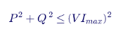
At reduced voltage the circle shrinks in proportion to voltage, and the controller's priority rules decide how the available current is shared between real and reactive output. In US practice, a combined STATCOM and storage asset may also participate in wholesale markets as a storage resource, which raises questions of registration, metering, market rules and NERC applicability that should be resolved early in the project.
12.3 Grid-forming STATCOMs
A grid-forming converter regulates its internal voltage magnitude and angle directly, behaving as a voltage source behind an impedance rather than a current source following a measured angle. A grid-forming STATCOM with some energy storage can provide a fast, inherent response to voltage and angle changes, contributing to system strength within its current rating. Its V–I characteristic in steady state can still include slope and limits, but its behavior within the first cycles of a disturbance differs from a grid-following design: it responds before any measurement and control loop acts.
Specifications for grid-forming capability are evolving in the US, with industry guidance from NERC and others. Projects considering grid-forming STATCOMs should define the performance expected (for example, response to phase jumps and voltage steps, current limiting behavior and stability in weak grids) in measurable terms.
How Keentel Engineering helps here: We evaluate hybrid configurations, energy-storage STATCOMs and grid-forming options against the actual system need, design the switching logic and current-priority rules, and verify performance in EMT simulation. We also help owners work through the regulatory and market questions that arise when a reactive device gains real power capability.
13. STATCOMs inside inverter-based generating plants
13.1 Why plants add STATCOMs
Solar, wind and battery storage plants provide reactive power from their inverters, but their reactive capability at the point of interconnection is reduced by the reactive losses of the collector system, the pad-mounted transformers and the main power transformer, and by the inverter's current limit when it is producing full real power. Many plants meet their interconnection requirements with inverters alone, by oversizing the inverter apparent-power rating. Others add a plant-level STATCOM, switched capacitors or both, particularly when:
- The inverters cannot meet the requirement at full output because of collector losses or a high-impedance main transformer.
- The interconnection agreement requires reactive support at zero output, for example at night for solar plants, and the inverters' night-time reactive capability is limited or not offered.
- The requirement is dynamic at a voltage range where the inverters' capability falls off.
- The plant replaces older equipment or must meet tightened requirements after a material modification.
13.2 US requirements
| Factor | Effect on transient |
|---|---|
| Point on wave of fault inception | Worst near a voltage zero crossing, when the stack capacitance holds maximum stored energy relative to the instantaneous voltage; mildest near a voltage peak |
| Total capacitance (C1 + C2) | Higher capacitance lowers the transient amplitude but can lengthen its duration; high-capacitance CVTs generally perform better |
| Ferroresonance suppression circuit type | Active (tuned L-C) circuits add a band-pass response and delay; passive (resistive) circuits produce less distortion |
| Secondary burden magnitude | Larger burden stores more energy and increases the transient |
| Secondary burden power factor | Inductive burdens make the transient more oscillatory at subnominal frequency |
| Step-down transformer excitation | Magnetizing current and core behavior shape the low-frequency component |
IEEE 2800 expresses reactive capability in terms of the plant's rated active power. At rated active power, the minimum reactive capability corresponds to a power factor of 0.95 in both directions, which is about 0.33 times the rated active power. The standard also defines reactive capability at reduced active power and over a voltage range at the reference point of applicability. The exact requirement applied to a specific plant depends on how the transmission provider has adopted the standard; engineers should read the interconnection agreement and the provider's requirements rather than assume.
Worked Example 11 — Does a 200 MW solar plant need a STATCOM?
Problem. System E is a 200 MW solar plant interconnecting at 230 kV. The requirement is 0.95 power factor leading and lagging at the high side of the plant substation at full output. The inverters are rated 215 MVA in total and produce 204 MW to deliver 200 MW at the POI after losses. The main power transformer is rated 200 MVA with 10 percent reactance; the pad-mounted transformers total 215 MVA with 6 percent reactance; the collector cables generate about 6 Mvar of charging. Estimate the plant's reactive capability at the POI and the size of any STATCOM needed.
Solution.
Required reactive power at the POI:

Inverter reactive capability at 204 MW within a 215 MVA rating:

Approximate transformer reactive losses at full output (I²X on each transformer's rating):
| Item | Reactive power (Mvar) |
|---|---|
| Inverter capability | +67.9 |
| Pad-mounted transformers (6% on 215 MVA, at full loading) | −12.9 |
| Main power transformer (10% on 200 MVA, at about 204 MVA through-flow) | −20.8 |
| Collector cable charging | +6.0 |
| Net lagging (supplying) capability at the POI | +40.2 |
| Requirement | +65.7 |
| Shortfall | 25.5 |
For the leading (absorbing) direction, the transformer losses help and the cable charging hurts: 67.9 + 12.9 + 20.8 − 6.0 ≈ 95.6 Mvar of absorption capability, which exceeds the requirement.
Interpretation. The plant meets the absorbing requirement easily but falls about 25 Mvar short in the supplying direction at full output. Options include a plant-level STATCOM of about ±30 Mvar (sized after accounting for its own coupling transformer and the voltage range), switched capacitors if the requirement allows a partly static solution, larger inverters, or a lower-impedance main transformer. A STATCOM is attractive where the requirement is dynamic, must be met at low voltage, or must be available at zero output; switched capacitors are cheaper where the requirement is mostly steady-state. The example uses simplified loss estimates. A real study models the collector system in detail, applies the requirement over the specified voltage range at the POI (where inverter current limits and transformer taps change the result), and checks the reactive capability at reduced output and at night.
13.3 Controlling a plant-level STATCOM
Inside a plant, the STATCOM normally does not regulate voltage on its own. The power plant controller (PPC) regulates voltage or reactive power at the POI and dispatches reactive orders to the inverters and the STATCOM. Coordination issues include:
- Allocation. Which resource moves first: the STATCOM (fast, but limited range) or the inverters (large range, but slower through the PPC loop)? A common approach lets the STATCOM respond to fast voltage changes with its own local control and lets the PPC slowly shift the steady-state burden to the inverters, the plant-level version of slow reset.
- Droop location. The plant's voltage droop is usually applied at the POI by the PPC. If the STATCOM also has a local slope, the combined droop must be understood and modeled.
- Speed. IEEE 2800 and many transmission provider requirements specify reactive response times at the POI. The combination of PPC update rates, communication latency and inverter response must meet them; the STATCOM can fill the fast part.
- Fault behavior. During faults, inverters and the STATCOM switch to their own fault ride-through logic. Their combined positive- and negative-sequence currents determine the plant's fault contribution and affect protection on the interconnecting line.
- Model validation. The plant model used for MOD-026 verification must include the STATCOM and its interaction with the PPC.
Keentel's companion article on power plant controller compliance covers PPC tuning and testing in detail.
How Keentel Engineering helps here: We calculate reactive capability at the POI across the full voltage and output range, determine whether a plant needs a STATCOM, switched capacitors or larger inverters, specify the device and its coordination with the power plant controller, and support model validation and testing for interconnection and NERC requirements. Our studies follow FERC Order 827, IEEE 2800 as adopted by the transmission provider and each provider's facility connection requirements.
14. Harmonics, losses, the coupling transformer and protection
14.1 Harmonics
STATCOMs produce far less harmonic distortion than SVCs with thyristor-controlled reactors, but they are not harmonic-free. The relevant points for specification and study:
- MMC STATCOMs synthesize a near-sinusoidal voltage from many small steps. Characteristic harmonics are low, and many designs need no harmonic filters at all. Small high-frequency components related to switching and submodule balancing remain.
- Two- and three-level PWM converters produce harmonics clustered around multiples of the switching frequency, usually requiring high-pass filters or larger phase reactors.
- Background harmonics and resonances. A STATCOM changes the network's harmonic impedance at its connection point. Its control can either damp or amplify existing harmonic voltages, depending on control bandwidth. The converter's harmonic impedance over frequency should be provided by the supplier and studied.
- Limits. In the US, IEEE 519 provides the recommended harmonic voltage and current limits at the point of common coupling. Transmission providers often specify their own limits and harmonic impedance envelopes. Keentel's companion article on harmonics and IEEE 519 explains the method.
14.2 Losses
| Zone | Typical protection |
|---|---|
| High-voltage connection and transformer | Transformer differential (87T), overcurrent (50/51), ground overcurrent (50N/51N), sudden pressure and gas relays, overexcitation (24) |
| Converter-side bus and reactors | Bus differential or overcurrent, reactor protection, ground fault detection on the ungrounded converter-side system |
| Converter valves and submodules | Internal overcurrent, overvoltage, temperature, cooling and submodule fault protection, with bypass and blocking logic |
| Switched capacitors and reactors in hybrids | Unbalance protection (60), overcurrent, overvoltage, reactor protection |
| System-level | Undervoltage and overvoltage (27/59), frequency (81) where required, breaker failure (50BF) |
For a STATCOM inside a generating plant, PRC-019 requires coordination between the voltage-regulating control limits and the protective relays of applicable generating facilities, and PRC-024 or PRC-029 sets ride-through expectations for the protection settings, depending on whether the facility is synchronous or inverter-based. Protection system maintenance falls under PRC-005 for BES protection systems. The STATCOM's own V–I characteristic should be the starting point for these coordination checks: protection must not trip the device inside the region of the characteristic the system relies on.
How Keentel Engineering helps here: We perform harmonic studies to IEEE 519 and transmission provider limits, evaluate losses over realistic operating profiles, specify coupling transformers, and design and set the protection for STATCOM and hybrid installations. For generating plants, we prepare PRC-019 coordination studies and PRC-024 or PRC-029 ride-through assessments that start from the device's actual characteristic.
15. Modeling the characteristic
15.1 Model types
| Model type | Purpose | How the V–I characteristic is represented |
|---|---|---|
| Power flow | Steady-state planning, Q–V and P–V analysis | Voltage-controlled reactive source with Mvar limits, or a switched shunt with continuous control; slope may or may not be represented |
| Positive-sequence dynamic (RMS) | Transient stability, FIDVR, voltage recovery | Generic or user-written model with slope, current limits, short-term overload, low-voltage logic and slow controls |
| Electromagnetic transient (EMT) | Control interactions, weak-grid stability, TOV, harmonics, fault behavior, protection | Detailed converter and control models, ideally the supplier's actual control code wrapped for the simulation platform |
| Real-time simulation with control replicas | Factory and site acceptance of controls | Actual controller hardware connected to a real-time network model |
15.2 Power flow representation
In power flow, a STATCOM is often modeled as a generator with zero real output and reactive limits equal to its rating, or as a switched shunt with continuous control. Two common errors:
- Constant-Mvar limits. A generator model with fixed Mvar limits delivers its full rating at any voltage, overstating a STATCOM at low voltage (where the real limit is current) and grossly overstating an SVC (where the limit is susceptance). Some programs offer voltage-dependent limits or dedicated FACTS device models; they should be used.
- No slope. Many power flow representations regulate voltage exactly. If the real device has a 3 percent slope, the power flow overstates the device's steady-state output and understates the voltage deviation. Where the program supports a regulation range or droop, it should be set to match.
15.3 Positive-sequence dynamic models
Generic models published for use across commercial planning programs represent SVCs and STATCOMs with slope, limits and a range of supplementary features. In the WECC generic model library, the static var system models include SVSMO1 (for SVCs), SVSMO2 (for thyristor-switched designs) and SVSMO3 (for STATCOMs); program-specific names add suffixes, and older program-specific models remain in use. The modeler's job is to set the parameters so that the model reproduces the actual device:
- Slope and reference, with the same base and the same form (current or reactive power) as the controller.
- Current limits, capacitive and inductive, at the correct terminals.
- Short-term overload magnitude, duration and recovery, if the model supports it.
- Low-voltage behavior, including thresholds for reduced current or blocking and the recovery ramp.
- Response time constants, matching measured step responses.
- Slow reset and switched shunt coordination, either within the model or by separate models of the switched elements.
Where a generic model cannot represent a feature that matters for the study, such as a specific overload logic or a particular fault strategy, the planner should either use a user-written model approved by the transmission planner or represent the feature conservatively.
15.4 EMT models
EMT models are now routine for STATCOMs on weak systems, near HVDC terminals or IBR clusters, and for protection and TOV studies. The preferred practice in the US is for the supplier to provide a model that uses the actual control code, with documentation, parameter sets matching the as-built settings and benchmark cases. Transmission providers increasingly require such models for interconnection and for inclusion in area EMT databases.
15.5 NERC modeling requirementss
| Standard | Relevance to STATCOMs |
|---|---|
| MOD-032 | Planning coordinators and transmission planners collect steady-state, dynamic and short-circuit model data from equipment owners, including transmission STATCOMs and SVCs |
| MOD-033 | Planning coordinators validate the system model against actual events, which exposes mismatches between modeled and actual compensator behavior |
| MOD-026 and MOD-027 (being consolidated as MOD-026-2) | Generator owners verify models of voltage control and active power control for applicable generating units, including plant-level reactive devices that are part of the plant's control |
| TPL-001 | Planning studies rely on accurate dynamic models of reactive devices, including their low-voltage behavior |
Keentel's companion articles on MOD-032 and MOD-033 discuss data submittals and validation in depth.
15.6 Validating the characteristic
Validation compares model behavior with field measurements. For a STATCOM, useful measurements include:
- Staged step tests, small reference steps (for example 1 to 2 percent) that show response time, overshoot and slope.
- Capability tests, which move the device to its capacitive and inductive limits at the available system voltage.
- Event recordings, from digital fault recorders and the device's own recorders, of natural disturbances such as faults and line trips; these show low-voltage and recovery behavior that cannot be safely staged.
- Slow control tests, showing slow reset and switched shunt coordination over several minutes.
A model that matches staged step tests but not fault recordings usually has wrong low-voltage or limiter parameters.
How Keentel Engineering helps here: We build and tune power flow, positive-sequence and EMT models of STATCOMs, SVCs and hybrid compensators, prepare MOD-032 data submittals, support MOD-026 verification for plant-level devices and validate models against staged tests and recorded events. When a generic model cannot represent a critical feature, we document the gap and develop a conservative or user-defined representation acceptable to the transmission planner.
16. Specifying the characteristic
16.1 Why the specification is where projects succeed or fail
A STATCOM specification is a contract that converts a planning study into equipment. In the US, IEEE 1052 provides a guide for specifying transmission STATCOM systems, and IEEE 1031 does the same for SVCs. Both emphasize functional requirements: the owner specifies what the device must do at the system level, and the supplier designs the equipment to do it. That approach works only if the functional requirements describe the characteristic completely.
16.2 Specification checklist for the V–I characteristic
| Item | What to state |
|---|---|
| Rating point | Continuous capacitive and inductive Mvar at a stated voltage at a stated terminal (normally the high-voltage bus) |
| Voltage range for rated current | Range of bus voltage over which continuous rated current is available in both directions |
| Reduced-current range | Behavior outside the rated voltage range, down to the minimum operating voltage and up to the maximum continuous voltage |
| Minimum operating voltage | Positive-sequence voltage below which current may be limited, the limiting characteristic, any blocking threshold and the recovery behavior |
| Short-term capacitive and inductive capability | Magnitude, duration, preload, voltage range and re-arming time |
| Slope | Adjustable range and resolution, base, form (current or reactive power), default setting |
| Reference | Adjustable range, ramp rate, remote and local control |
| Deadband | Availability and adjustable range |
| Control modes | Voltage, reactive power, power factor and external current reference, and the transfer between them |
| Response | Closed-loop response time and overshoot for a defined voltage step at stated minimum and maximum system strengths |
| Slow reset and switched shunt control | Thresholds, delays, priorities, minimum on and off times |
| Gain supervision | Required function and its behavior |
| Power oscillation damping | Input signals, gain range and output limits |
| Fault behavior | Positive- and negative-sequence current strategy during faults; recovery ramp; behavior for reclosing |
| TOV capability | Voltage and duration capability and required inductive response |
| System strength range | Minimum and maximum short-circuit levels, and network impedance data for EMT studies |
| Harmonics | Emission limits, background harmonics, harmonic impedance envelopes |
| Losses | Evaluation points and capitalization rates |
| Availability and redundancy | Target availability, redundancy for submodules, cooling and control |
| Ambient and altitude | Site ranges for rated output |
| Models | Power flow, positive-sequence and EMT models, with benchmark cases and update obligations |
| Testing | Factory, real-time simulation, site and staged performance tests |
16.3 Common specification gaps
From Keentel's reviews of STATCOM and SVC specifications and bids, the most frequent gaps are:
- Rating at the converter terminals instead of the high-voltage bus, as in Worked Example 2.
- Short-term capability stated without preload or voltage range, so that the bid's "1.3 pu for 2 s" applies only from no load at nominal voltage.
- No minimum operating voltage, leaving the low-voltage behavior to the supplier's default.
- Response time defined ambiguously, for example without stating the step size, the measured quantity or the system strength.
- Slope range without a base, causing a factor-of-two error when entered into the planning model.
- No EMT model requirement, or a requirement without benchmark cases and update obligations after control changes.
- No requirement for slow reset coordination with existing switched shunts at the station.
16.4 Bid evaluation
Comparing STATCOM bids requires putting each supplier's characteristic on the same basis. Keentel's bid evaluation approach:
1. Convert each bid to the same rating point (high-voltage bus at a stated voltage), including transformer reactive losses and auxiliary loads.
2. Plot each characteristic in V–I and V–Q form, including short-term and low-voltage behavior.
3. Re-run the critical dynamic cases with each bidder's characteristic to confirm that performance criteria are met.
4. Evaluate losses at the specified operating points with capitalized values.
5. Compare lifecycle costs, including maintenance, spare parts, availability guarantees and expected refurbishment of control systems.
17. Testing and commissioning
17.1 Factory testing
Factory testing of valves, submodules, transformers and reactors follows the applicable equipment standards and the supplier's type and routine test programs. For the characteristic itself, the most valuable factory test is a closed-loop test of the actual control and protection system against a real-time digital simulation of the network. Typical real-time test cases:
- Voltage reference steps of several sizes at minimum and maximum system strength.
- System voltage steps caused by line switching in the simulated network.
- Faults of all types at several locations and clearing times, with and without reclosing.
- Low-voltage operation near and below the minimum operating voltage.
- Short-term overload and re-arming.
- TOV events such as load rejection.
- Slow reset and switched shunt coordination over minutes of simulated time.
- Gain supervision at the weakest system strength.
- Control mode transfers and loss of communication.
The results also provide the benchmark cases against which the positive-sequence and EMT models are validated.
17.2 Site acceptance and energization
Site acceptance testing verifies the installation, wiring, protection and control system before and during energization. Steps typically include protection relay testing, control and interlock checks, cooling system tests, transformer energization, converter deblocking at low output and gradual increase to rated output in both directions.
17.3 Staged performance tests
After energization, staged tests verify the characteristic on the real system:
| Test | What it verifies |
|---|---|
| Reference step tests (small steps in both directions) | Response time, overshoot, settling and slope |
| Slope verification | Steady-state output versus voltage deviation along the sloped line |
| Capacitive and inductive capability | Output at the current limits at the available system voltage |
| Mode transfer | Bumpless transfer between voltage, var and other modes |
| Slow reset | Switching of shunts and return of output to the target band |
| Switched shunt coordination | Voltage step and recovery when a bank switches |
| Power oscillation damping | Response to a test signal if POD is enabled |
Capacitive capability at low voltage, short-term overload and fault behavior usually cannot be staged safely on a transmission system. They are verified in factory real-time tests and later confirmed from natural disturbance recordings.
17.4 Ongoing verification
A STATCOM's characteristic should be monitored throughout its life. Fault recorders at the station and the device's own event logs capture its response to natural events. Comparing these recordings with the model is the most effective form of continuing validation, and is directly useful for MOD-033 system model validation and, for plant-level devices, MOD-026 re-verification.
How Keentel Engineering helps here: We write and review STATCOM specifications to IEEE 1052 and SVC specifications to IEEE 1031, evaluate bids on an equal-performance basis, witness factory real-time simulation tests, prepare and witness staged commissioning tests and analyze event recordings to confirm that the installed characteristic matches the model and the specification.
18. Operation, maintenance and lifecycle
18.1 Operating practices
- Voltage schedules. System operators set the STATCOM reference and slow reset targets in coordination with generator voltage schedules under VAR-001 and VAR-002.
- Reserve monitoring. Operators should see the device's dynamic reserve, not just its output. A STATCOM sitting at 80 percent capacitive in steady state is a warning that slow reset or switched shunts are not doing their job.
- Outage coordination. A STATCOM outage can reduce transfer limits or require operating restrictions. Planned outages should be studied like other reactive resource outages.
- Event review. Each significant disturbance is an opportunity to compare actual and modeled response.
18.2 Maintenance
| Subsystem | Typical maintenance focus |
|---|---|
| Valves and submodules | Inspection, replacement of failed submodules from spares, firmware management |
| Cooling | Coolant quality, pumps, fans, heat exchangers, leak detection |
| Control and protection | Software version control, backup of settings, cybersecurity patching where applicable, PRC-005 testing of protection systems |
| Transformer and reactors | Oil testing, dissolved gas analysis, bushings, tap changer if present |
| Switched shunts | Capacitor unit testing, unbalance protection, switching device maintenance |
18.3 Lifecycle
Power semiconductors and capacitors are long-lived when operated within their ratings, but control and protection hardware ages faster and is often replaced or upgraded mid-life. Cooling systems are a frequent source of forced outages. A mid-life review should re-examine the characteristic against the system's current needs, which may have changed substantially with new generation and load, and should update models accordingly.
18.4 Refurbishing or replacing an older compensator
Many US SVCs installed in the 1980s and 1990s, and some early STATCOMs, are approaching the end of their control system and valve lives. Owners face a choice between refurbishing the existing device, replacing it with a modern STATCOM or hybrid, or retiring it in favor of synchronous condensers or other solutions. The V–I characteristic is the right starting point for that decision:
- Re-establish the need. The system around an older device has usually changed: generation has retired or been added, inverter-based resources have arrived, loads have grown or shifted. The characteristic that was right twenty-five years ago may be too small, too slow at low voltage or poorly placed today.
- Measure the existing characteristic. Event recordings and staged tests show what the device actually does, which may differ from its original specification after years of component replacements and setting changes.
- Compare options on equal performance. A refurbished SVC with new controls keeps its V² behavior at low voltage. A replacement STATCOM of the same nameplate gives more support during sags but may need a different footprint and transformer. A hybrid may reuse existing capacitor banks.
- Plan the outage. Replacing a dynamic reactive device takes it out of service for months. Interim operating measures, such as temporary capacitor banks, operating restrictions or generation commitments, must be studied.
- Update models and compliance records. The new characteristic must flow into MOD-032 data, planning cases, protection settings and operating procedures.
19. Standards and compliance map
| Standard or document | Relevance |
|---|---|
| IEEE 1052 | Guide for specification of transmission STATCOM systems |
| IEEE 1031 | Guide for functional specification of transmission static var compensators |
| IEEE 2800 | IBR performance, including reactive capability and voltage control at the reference point of applicability |
| IEEE 519 | Harmonic control limits at the point of common coupling |
| IEEE C57.12 series | Power transformer requirements for coupling transformers |
| IEEE C37 series | Protective relaying and switchgear for the installation |
| IEEE C62 series | Surge protection and insulation coordination |
| NERC TPL-001 | Transmission planning performance requirements, including voltage criteria |
| NERC MOD-032, MOD-033 | Model data and model validation |
| NERC MOD-026, MOD-027 (MOD-026-2) | Model verification for generating facilities, including plant-level reactive devices |
| NERC VAR-001, VAR-002 | Voltage and reactive control by transmission operators and generator operators |
| NERC PRC-005, PRC-019, PRC-024, PRC-029 | Protection maintenance, coordination of voltage controls with protection, ride-through |
| NERC FAC-002 | Facility interconnection studies |
| FERC Orders 827 and 2023 | Reactive power requirements for non-synchronous generators; interconnection process reform |
| NESC (ANSI C2) | Safety rules for the substation and its clearances |
| NEC (NFPA 70) and NFPA 70E | Building and auxiliary systems wiring and electrical safety in work practices |
20. Choosing a solution: putting the characteristic to work
| If the system need is mainly | Consider first | Why |
|---|---|---|
| Steady-state reactive deficit that varies daily | Switched capacitors and reactors | Lowest cost per Mvar; adequate speed |
| Fast voltage support during faults and recovery, deep sags, FIDVR | STATCOM, or hybrid STATCOM with switched shunts | Current-limited output holds up at low voltage; fast response |
| Fast support near normal voltage, high inductive duty | SVC or STATCOM | Near 1.0 pu the two are similar; SVC's V² behavior helps on the inductive side |
| System strength, inertia, fault current for protection and IBR stability | Synchronous condenser or grid-forming converter | Grid-following STATCOMs do not add system strength in the protection sense |
| Flicker and fast load compensation | STATCOM | Speed and bandwidth |
| IBR plant reactive shortfall | Larger inverters, switched capacitors or plant-level STATCOM, depending on dynamic and low-voltage requirements | Least-cost combination that meets the interconnection requirement |
| Real power and frequency services as well as voltage | STATCOM with storage, or BESS with grid-forming controls | Combined capability within a shared current limit |
Every row requires confirmation by study. The value of understanding the V–I characteristic is that it lets owners and planners ask the right questions of each option: how much does it deliver at the voltages that matter, for how long, how does it share with its neighbors, and does the model tell the truth about it?
21. Twelve questions to ask about any STATCOM characteristic
Whether reviewing a supplier's bid, an interconnection customer's data submittal or an existing device's documentation, these questions expose most of the gaps between the characteristic that was drawn and the one that will perform:
1. At which terminals is the rating stated, and at what voltage? If it is at the converter terminals, what does the device deliver at the high-voltage bus after transformer losses and auxiliary loads?
2. Over what voltage range is full continuous current available in each direction? Where does the capacitive limit bend at high voltage and the inductive limit at low voltage?
3. What is the minimum operating voltage? What happens below it, for balanced and unbalanced faults, and how quickly does the device recover once voltage returns?
4. What short-term capability exists in each direction? State magnitude, duration, preload, voltage range and re-arming time.
5. What slope range, base and form does the controller use? Is the slope applied to current or to reactive power, and what is the default?
6. What control modes are available, and how are transfers between them handled?
7. Is there slow reset, and what does it control? Which external capacitors and reactors does it coordinate, with what thresholds and delays?
8. How is response time defined and demonstrated? For what step, at what system strength, measured how?
9. What is the fault strategy? Positive- and negative-sequence current priorities, behavior during and after faults, and reclosing.
10. What protection could trip the device inside the region of the characteristic the system relies on? Undervoltage, overvoltage, overcurrent and cooling trips should all sit outside it.
11. Which models represent all of this? Power flow, positive-sequence and EMT models, their parameter sets, benchmark cases and update obligations.
12. How will each part of the characteristic be verified? Factory real-time tests, staged site tests and event-based validation, with acceptance tolerances.
A complete answer to these twelve questions is, in effect, a complete description of the device's V–I characteristic. An incomplete answer is a risk that will surface eventually, either in a study, in a test or during an event.
How Keentel Engineering helps here: We use this checklist on every compensator project we review, whether we are acting as owner's engineer, reviewing an interconnection customer's data for a transmission provider or investigating a performance issue after an event. Clients receive a gap list with specific requests to the supplier and a clear statement of which gaps affect planning, protection or compliance.
Part C — Case Studies
Case Study 1 — A Southeastern load pocket: sizing for the voltage that matters
Background. A transmission owner in the Southeastern US served a fast-growing suburban area through two 230 kV lines and several 115 kV ties. Summer peak load was dominated by residential air conditioning. Dynamic simulations with composite load models showed that a three-phase fault on one 230 kV line with delayed clearing caused FIDVR: voltage at the main 230/115 kV substation stayed below 0.8 pu for more than two seconds, violating the planner's transient voltage criteria. An initial proposal called for a ±200 Mvar SVC, sized from a steady-state Q–V curve that showed a 180 Mvar post-contingency deficit at 0.97 pu.
What Keentel did. Keentel was engaged as owner's engineer to review the solution. We re-ran the dynamic studies with the planner's composite load model, representing an SVC and a STATCOM with their actual low-voltage behavior, slope, response time and, for the STATCOM, an assumed minimum operating voltage of 0.3 pu with no short-term overload. Key findings:
- The steady-state need and the dynamic need were different. The 180 Mvar steady-state deficit at 0.97 pu was real, but it lasted for minutes and could be met with switched capacitors under slow control. The criteria violation occurred in the first two seconds after the fault, with bus voltage between 0.65 and 0.8 pu.
- At those voltages the SVC underperformed. In the critical period, a ±200 Mvar SVC delivered roughly 85 to 130 Mvar; a ±200 Mvar STATCOM delivered 130 to 160 Mvar. Only the STATCOM case met the transient voltage criteria, and only with a few hundredths of a pu of margin.
- A hybrid was cheaper than a larger converter. A ±150 Mvar STATCOM with two 75 Mvar switched capacitor banks under slow reset met both the transient criteria and the steady-state deficit. The capacitors handled the post-contingency steady state; the STATCOM was kept near zero output by slow reset and so started each event with its full range.
- The specification needed a low-voltage clause. We added a requirement for rated current down to 0.3 pu positive-sequence voltage, a 3 percent default slope on the STATCOM rating, a stated rating at the 230 kV bus and an EMT model with benchmark cases.
Outcome. The utility adopted the hybrid design. Bid evaluation on the specified basis showed that two of the three bidders' standard designs reduced current below 0.4 pu; one bidder modified its control to meet the requirement. Commissioning step tests matched the model within the stated tolerances, and a later natural fault event showed the STATCOM holding full capacitive current at about 0.6 pu for roughly 150 milliseconds before recovery, consistent with the model.
Lessons. Size dynamic devices at the voltage where the criteria are violated, not at the steady-state target voltage. Separate the steady-state and dynamic needs. Specify the low-voltage characteristic explicitly.
Case Study 2 — A Texas wind and solar hub: two compensators fighting
Background. In a part of Texas with high concentrations of wind and solar generation, a 345 kV substation hosted a 200 MW wind plant with a plant-level ±60 Mvar STATCOM and, two buses away, a utility-owned ±150 Mvar SVC that had been in service for many years. Operators noticed slow oscillations in reactive output between the two devices during low-load night hours, with the STATCOM moving toward its inductive limit while the SVC moved capacitive, and the 345 kV voltage drifting slightly. Occasionally the plant's STATCOM hit its limit, and the plant's power plant controller then pushed the wind turbines to absorb reactive power, reducing their capability for the morning ramp.
What Keentel did. Keentel was engaged by the plant owner to investigate. We collected settings from both devices and the PPC and reproduced the behavior in a positive-sequence model with long-term dynamics, then confirmed key details in EMT. Findings:
- References were inconsistent.The SVC was set to regulate its bus at 1.02 pu, while the plant's voltage schedule at its POI, two buses away, was 1.00 pu. In the electrical distance between them, the two targets could not both be met without one device absorbing and the other supplying.
- The plant's effective slope was very small.The PPC applied a 1 percent droop at the POI, and the STATCOM, slaved to the PPC, effectively inherited it. The SVC had a 5 percent slope. With the smaller slope, the plant's devices did most of the fighting.
- The PPC and SVC slow controls had overlapping time constants, producing a slow, poorly damped exchange between the two.
Outcome. Working with the transmission operator, Keentel recommended aligning the voltage schedules, increasing the plant's droop at the POI to 4 percent (within the provider's allowed range), adding a deadband to the plant's slow reactive allocation and adjusting the PPC's slow reset time constant to separate it from the SVC's. After implementation, the circulating reactive power fell from several tens of Mvar to a few Mvar, the oscillations disappeared and the plant's dynamic reserve at dawn improved. Updated settings were documented for the plant's MOD-026 model verification and reported in the transmission planner's model data.
Lessons. Slopes and references must be coordinated across owners. A small slope is not "better regulation" if a neighboring device is regulating to a different target. Long-term dynamic simulation reveals interactions that short transient stability runs miss.
Case Study 3 — A Mid-Atlantic data center campus: the rating that was in the wrong place
Background. A developer building a large data center campus in the Mid-Atlantic region connected to the utility at 230 kV through two 230/34.5 kV transformers. The utility's facility connection requirements included a voltage performance requirement at the 230 kV point of interconnection: during and after specified faults on the 230 kV system, the campus must not draw reactive power that worsened voltage recovery, and it must be capable of a defined reactive support range at the POI. The developer's design-build contractor procured a ±80 Mvar STATCOM, connected at 34.5 kV, to meet the requirement and to help ride-through of the campus's sensitive loads.
What Keentel did. Keentel was engaged by the developer as owner's engineer late in the design stage to review compliance with the utility requirements. We found:
- The rating was at the wrong terminals. The STATCOM was rated ±80 Mvar at its 34.5 kV terminals. Between the STATCOM and the POI were a 34.5 kV cable system and one of the 230/34.5 kV transformers with about 11 percent reactance on 120 MVA. At full capacitive output, those elements absorbed roughly 6 to 8 Mvar, so the capacitive support at the POI fell short of the requirement by several Mvar.
- Short-term overload was quoted for no preload. The supplier's data showed 1.2 pu for 2 s, but only from zero output. Under the campus's normal operation, the STATCOM held about 30 percent capacitive output to offset the campus's reactive demand, which reduced the available overload duration.
- Fault behavior was unknown. The supplier's standard fault strategy reduced output below 0.4 pu, while the utility's requirement covered faults that depressed the 34.5 kV bus below that level.
Outcome. Keentel worked with the developer, contractor and supplier to resolve the issues before equipment shipment. The supplier confirmed that the converter could deliver about 10 percent more current within its thermal design at the site's ambient conditions, which together with a revised transformer tap setting closed the POI shortfall. A small switched capacitor bank was added at 34.5 kV under slow reset control to take over the campus's steady-state reactive demand, returning the STATCOM's steady-state output to near zero and restoring its overload capability. The supplier provided a revised low-voltage control setting and an EMT model that demonstrated compliance with the utility's fault cases. The utility accepted the revised design after reviewing Keentel's study report.
Lessons. For large loads as well as generators, reactive requirements apply at the POI, not at the device. Overload capability depends on preload, and steady-state reactive demand consumes it. Late design reviews are expensive; early ones are cheap.
Part D — Frequently Asked Questions
1. What does the STATCOM V–I characteristic show?
It shows the steady-state relationship between the STATCOM's terminal voltage and its reactive current. In the control range, the device follows a sloped line through its reference voltage. At the ends, vertical lines mark the maximum continuous capacitive and inductive currents. Many diagrams add short-term overload limits and a low-voltage region where the converter may limit or block. The characteristic is the starting point for sizing, specification, modeling, protection coordination and testing.
2. Why is capacitive current shown on the left and inductive on the right?
It is a convention inherited from SVC and FACTS textbooks, in which the capacitive (supplying) side is drawn as negative current. Power flow and stability programs normally use generator convention, in which supplying reactive power is positive Mvar. Neither is wrong, but mixing them causes sign errors in models and settings. Every specification, model and test report should state its convention.
3. Does a STATCOM really deliver constant current at reduced voltage?
Within its design range, yes: at its capacitive limit it holds the maximum current, so its reactive output falls only in proportion to voltage. But the range has a lower bound. Below a minimum operating voltage, which depends on the design and is often specified around 0.2 to 0.4 pu, the converter may reduce its current or block because of synchronization, control or protection limits. The actual low-voltage characteristic must be obtained from the supplier and represented in models.
4. How much more reactive power does a STATCOM provide than an SVC during a voltage sag?
For equal nameplate at 1.0 pu voltage, the ratio is 1/V. At 0.9 pu the STATCOM provides 11 percent more, at 0.7 pu 43 percent more, at 0.5 pu twice as much. Above 1.0 pu the SVC actually provides slightly more capacitive output. The right comparison is equal performance at the voltage that matters for the planning criteria, not equal nameplate.
5. What is the slope, and why not set it to zero?
The slope is the deliberate change in regulated voltage with compensator current, typically 1 to 5 percent on the compensator rating. A zero slope would make the device fight neighboring regulators, swing to its limits for small disturbances, prevent slower devices such as tap changers from taking over and reduce the voltage loop's stability margin on weak systems. Worked Example 5 shows two compensators with nearly zero slope and a 0.5 percent reference mismatch driving each other to opposite limits.
6. What slope value should I use?
Most transmission STATCOMs and SVCs use 2 to 4 percent, often 3 percent, on their own rating. Weak or radial systems may justify up to 5 percent; load compensators may use less. The right value comes from a coordination study that considers the devices sharing the area, their ratings, the desired sharing, steady-state utilization, stability across system strengths and interaction with slower controls.
7. On what base is the slope expressed?
Normally on the compensator's own rating at 1.0 pu voltage. A 3 percent slope on a 150 Mvar device is 0.03 pu on 150 MVA, which is 0.02 pu on a 100 MVA system base. Planning models may require the slope on a different base or in a different form, such as reactive power rather than current. Converting incorrectly is a common error.
8. How is the operating point determined?
By the intersection of the compensator's sloped characteristic with the system's Thevenin line. The STATCOM's current equals the difference between the system's open-circuit voltage and the reference, divided by the sum of the system reactance and the slope reactance, subject to the current limits. A strong system with a small deficit uses little of the range; a weak system or a large deficit uses more, until the limit is reached.
9. What is slow reset, and why does it matter?
Slow reset is a supervisory control that drives the STATCOM's steady-state output back toward a target band near zero over seconds to minutes, by adjusting the reference within limits or by switching external capacitors and reactors. It keeps the fast converter range available for disturbances. Without it, a STATCOM can spend its capacity on slow, steady-state voltage support and have little left when a fault occurs.
10. What sets a STATCOM's continuous current limit?
Mainly the thermal capability of the semiconductor valves and the cooling system, with contributions from the phase reactors, coupling transformer, bus work and, in MMC designs, submodule capacitor voltage ripple. The rating is stated at a maximum ambient temperature and may be lower in extreme heat or at high altitude.
11. Is the transient overload always available for less than one second?Question
No. Short-term overload magnitude and duration are design-specific. Some STATCOMs have little or no capacitive overload; others can carry about 1.2 to 1.5 pu for a fraction of a second to several seconds. The duration depends strongly on preload: in Worked Example 7, a 1.3 pu overload lasts about 2.3 seconds from no load but under 1 second from full load. Specifications should state magnitude, duration, preload, voltage range and re-arming time.
Q12. Are capacitive and inductive overloads the same?uestion
Not necessarily. Capacitive overload requires a higher converter voltage, which modulation and submodule voltage limits may restrict. Inductive overload at high voltage stresses valves, submodule capacitors and the coupling transformer's core differently. Each direction should be specified and tested separately.
13. Does an SVC have a transient rating?
On the inductive side, yes, in many designs: the thyristor-controlled reactor can carry short-term overcurrent at high voltage for TOV control. On the capacitive side, an SVC at full susceptance is a fixed capacitor with no overload in the usual sense. Both technologies therefore need explicit short-term requirements in their specifications.
14. How does the coupling transformer affect the characteristic?
It consumes reactive power proportional to the square of current, so capacitive output at the high-voltage bus is lower than at the converter terminals, and inductive absorption is higher. It also determines the converter voltage needed for full current. In Worked Example 2, a 12 percent transformer reduces a 150 Mvar converter's capacitive output at the 230 kV bus to about 132 Mvar. Ratings should be stated at the high-voltage bus.
15. What happens to a STATCOM during an unbalanced fault?
Its positive-sequence voltage drops less than the faulted phase voltage. Depending on its control, it may inject only positive-sequence current or both positive- and negative-sequence currents. Injecting negative-sequence current helps reduce voltage unbalance but uses part of the phase current limit, so less positive-sequence current is available. Delta-connected cascaded designs must also manage cell energy balance. The behavior affects nearby protection and should be represented in EMT studies.
16. How fast does a STATCOM respond?
The inner current loop acts within milliseconds, but the meaningful figure is the closed-loop voltage response, typically about one to two cycles (roughly 15 to 35 milliseconds) to reach 90 percent of a step change for transmission STATCOMs, compared with typically two to five cycles for SVCs. Actual response depends on regulator gain and system strength. Specifications should define the response time precisely: step size, measured quantity and system strength.
17. Why does the STATCOM's behavior change when the grid weakens?
The voltage change per Mvar is inversely proportional to the short-circuit level, so the voltage regulator's effective gain rises as the grid weakens. A regulator tuned for the intact system may oscillate after line outages. The PLL can also become less stable at low SCR. Gain supervision, adaptive gain, conservative tuning and a modestly larger slope are common remedies, verified by EMT studies at the weakest credible case.
18. Does a STATCOM increase system strength?
Not in the protection sense. A grid-following STATCOM supplies limited fault current, no inertia and does not raise the short-circuit level that other converters and protection rely on. It improves voltage behavior through fast control. Where system strength is the problem, synchronous condensers, grid-forming converters or transmission reinforcement are the usual solutions.
19. What is a hybrid STATCOM?
A STATCOM combined with mechanically or thyristor-switched capacitors and reactors, or fixed filters. The switched elements extend the total range at low cost, while the converter provides fast, continuous control and low-voltage support. Slow reset logic coordinates them so that the converter stays near zero output in steady state. Switched capacitors' output falls with V² during sags, so the converter carries most of the dynamic burden.
20. Can a STATCOM provide real power?
A conventional STATCOM exchanges only enough real power to cover its losses. A STATCOM with energy storage, or an E-STATCOM, can also exchange real power for frequency response, power oscillation damping and other services. Real and reactive current then share the same current limit, so priority rules determine what is available during an event.
21. How is a STATCOM modeled in power flow?
Usually as a voltage-controlled reactive source with Mvar limits or as a continuously controlled switched shunt. Fixed-Mvar limits overstate low-voltage capability, and exact voltage regulation ignores the slope. Where the program supports it, voltage-dependent limits and a regulation range or droop should be used to reflect the real characteristic.
22. Which dynamic models are used for STATCOMs?
Generic models such as those in the WECC library (for example the static var system model intended for STATCOMs, named SVSMO3 in the generic library with program-specific suffixes), program-specific models and user-written models. Parameters must match the actual slope, limits, overload logic, low-voltage behavior and response. EMT models, ideally using the supplier's actual control code, are needed for weak-grid, interaction, TOV and protection studies.
23. How does FERC Order 827 affect STATCOM use at renewable plants?
Order 827 requires newly interconnecting non-synchronous generators to provide dynamic reactive power within a 0.95 leading to 0.95 lagging power factor range at the high side of the generator substation. Collector and transformer reactive losses can leave the inverters short, as Worked Example 11 shows, and a plant-level STATCOM is one way to close the gap. Larger inverters or switched capacitors may be cheaper, depending on how much of the requirement must be dynamic.
24. How does IEEE 2800 relate to STATCOMs?
IEEE 2800 sets performance requirements for inverter-based resources at the reference point of applicability, including reactive capability, voltage control, ride-through and fault current behavior. A plant-level STATCOM is part of the plant's capability and must perform consistently with the plant's obligations. The requirements that apply to a specific plant depend on how the transmission provider has adopted the standard.
25. Which NERC standards apply to a transmission STATCOM?
Relevant standards include TPL-001 for planning studies that rely on the device, MOD-032 for model data, MOD-033 for model validation, VAR-001 for transmission operator voltage control, PRC-005 for maintenance of its protection systems where they are BES protection systems, and FAC-002 for interconnection studies. Plant-level devices in generating facilities also fall under generator-related standards such as VAR-002, MOD-026 and MOD-027 (being consolidated as MOD-026-2), PRC-019 and PRC-024 or PRC-029, depending on registration and applicability.
26. How do I size a STATCOM for a voltage problem?
Use P–V and Q–V analysis to find the steady-state reactive deficit under contingencies, then time-domain dynamic studies with composite load models to find the dynamic need during the transient period. Separate the steady-state need, often best met with switched capacitors, from the dynamic need, which justifies a STATCOM. Size the STATCOM at the voltage where the criteria are at risk, include coupling transformer losses and check the slope's effect on steady-state utilization.
27. Can a STATCOM fix FIDVR?
It helps, but rarely solves FIDVR alone. Stalled motors absorb very large amounts of reactive power; in Worked Example 9, a 300 Mvar STATCOM raised a stalled-motor bus only from 0.76 to 0.88 pu. Effective mitigation combines dynamic reactive support with faster fault clearing, load-side measures and, where appropriate, under-voltage load shedding.
28. What should a STATCOM specification include about the characteristic?
Rating at a stated terminal and voltage; the voltage range for rated current; the minimum operating voltage and behavior below it; short-term capability with magnitude, duration, preload, voltage range and re-arming; slope range and base; control modes, slow reset and deadband; response time definitions; fault strategy; TOV capability; system strength range; harmonic, loss and availability requirements; and model and test obligations. IEEE 1052 provides a framework for transmission STATCOM specifications.
29. How is the characteristic verified after installation?
Factory real-time simulation tests verify control behavior across faults, low voltage, overload and weak-grid conditions. Staged site tests verify slope, response time, capability at available voltages, mode transfers and slow reset. Low-voltage behavior and overload are then confirmed from natural disturbance recordings, which also support MOD-033 validation and, for plant devices, MOD-026 verification.
30. When should I choose an SVC, a synchronous condenser or a STATCOM?
Choose based on the need. For deep-sag support, fast response and compact footprint, a STATCOM or hybrid STATCOM usually wins. Near normal voltage, or where large inductive duty dominates, an SVC can be competitive, especially for refurbishments. Where system strength, inertia or fault current are needed, a synchronous condenser or grid-forming converter is the right tool. Many projects combine technologies. In each case, compare options on equal performance at the voltages that matter, over the full lifecycle.
How Keentel Engineering Helps
Keentel Engineering is a US power system engineering firm that plans, studies, designs and commissions electrical systems for utilities, transmission owners, independent power producers, large-load customers such as data centers, industrial plants and campuses, from 4 kV distribution to 765 kV transmission. Dynamic reactive power and voltage control is one of our core disciplines.
For STATCOMs, SVCs, synchronous condensers and hybrid compensators, our services include:
- Reactive power and voltage stability studies: P–V and Q–V analysis, contingency screening, transient voltage recovery and FIDVR studies with composite load models, to TPL-001 and regional criteria.
- STATCOM and SVC sizing and technology selection: separating steady-state and dynamic needs, comparing STATCOM, SVC, synchronous condenser, hybrid and grid-forming options on equal-performance terms, and recommending location, rating, slope and short-term capability.
- Specification and bid evaluation: functional specifications to IEEE 1052 and IEEE 1031, with complete V–I characteristic requirements, and bid evaluation that puts each supplier's characteristic, losses and lifecycle cost on the same basis.
- Owner's engineer services: independent technical oversight from concept through design, factory testing, installation, commissioning and warranty, for utilities, developers and large-load owners.
- EMT studies: PSCAD and other EMT studies of control interactions, weak-grid stability, TOV, harmonics, fault behavior and protection performance, using supplier control-code models where available.
- Planning model development: power flow and dynamic models in PSS/E and PSLF, parameter tuning of generic models, user-written model reviews and model benchmarking against EMT and test results.
- NERC model verification and data: MOD-032 data submittals, MOD-033 validation support, and MOD-026 and MOD-027 model verification (including the consolidated MOD-026-2 as it takes effect) for generating plants with plant-level reactive devices.
- Interconnection studies and IBR compliance: reactive capability studies at the POI under FERC Order 827, IEEE 2800 assessments as adopted by the transmission provider, power plant controller coordination and interconnection study support under the FERC Order 2023 process.
- Large-load interconnection: voltage performance studies, reactive compensation design and utility requirement compliance for data center campuses and industrial facilities.
- Harmonic studies: IEEE 519 compliance, harmonic impedance and resonance analysis and filter design.
- Protection and control: protection design and settings for STATCOM, SVC and hybrid installations, coupling transformers and switched shunts; PRC-019 coordination studies; PRC-024 and PRC-029 ride-through assessments; PRC-005 maintenance programs.
- Commissioning and testing: test plans, witness of factory real-time simulation tests, staged site performance tests and post-event analysis of recordings.
- NERC compliance programs: VAR-001 and VAR-002 support, documentation and audit readiness for transmission and generator entities.
- Substation and transmission design: physical, electrical and protection and control design for compensator installations and interconnection substations.
Why Clients Choose Keentel
- Study-to-steel expertise: our engineers connect planning studies, specifications, models, protection and commissioning, so the characteristic the planner assumed is the characteristic that gets built and tested.
- Independent advice: we are not tied to any equipment supplier, so our recommendations follow the engineering and the client's interests.
- US standards fluency: daily work with NERC TPL, MOD, VAR and PRC standards, IEEE 1052, 1031, 2800 and 519, FERC interconnection requirements, NESC and NEC.
- Auditable deliverables: every rating, slope and setting traces back to a documented study case, with calculations that reviewers and auditors can follow.
- EMT and positive-sequence depth: we model both, and we know when each is needed.
- Full voltage range: from 4.16 kV plant distribution to 765 kV transmission, including the interconnection facilities that connect new generation and large loads to the grid.
Talk to an Engineer
Planning a STATCOM, upgrading an aging SVC, closing a reactive shortfall at a solar, wind or storage plant, or meeting a utility's voltage performance requirements for a data center campus? Keentel Engineering can review your system and deliver a documented, defensible answer.
- Phone: (813) 389-7871
- Email: contact@keentelengineering.com
- Book a 15-minute call: calendly.com/keentel-engineering/15min
References
- IEEE Std 1052, IEEE Guide for Specification of Transmission Static Synchronous Compensator (STATCOM) Systems.
- IEEE Std 1031, IEEE Guide for the Functional Specification of Transmission Static Var Compensators.
- IEEE Std 2800-2022, IEEE Standard for Interconnection and Interoperability of Inverter-Based Resources (IBRs) Interconnecting with Associated Transmission Electric Power Systems.
- IEEE Std 519, IEEE Standard for Harmonic Control in Electric Power Systems.
- IEEE Std C57.12.00, IEEE Standard for General Requirements for Liquid-Immersed Distribution, Power, and Regulating Transformers.
- NERC Reliability Standards TPL-001, MOD-026, MOD-027, MOD-032, MOD-033, VAR-001, VAR-002, PRC-005, PRC-019, PRC-024, PRC-029 and FAC-002, current effective versions.
- FERC Order No. 827, Reactive Power Requirements for Non-Synchronous Generation, 2016.
- FERC Order No. 2023, Improvements to Generator Interconnection Procedures and Agreements, 2023.
- WECC, Static Var System Generic Models (SVSMO1, SVSMO2, SVSMO3) model specifications.
- N. G. Hingorani and L. Gyugyi, Understanding FACTS: Concepts and Technology of Flexible AC Transmission Systems, IEEE Press.
- R. M. Mathur and R. K. Varma, Thyristor-Based FACTS Controllers for Electrical Transmission Systems, IEEE Press and Wiley.
- P. Kundur, Power System Stability and Control, McGraw-Hill.
- T. J. E. Miller (ed.), Reactive Power Control in Electric Systems, Wiley.
- C. W. Taylor, Power System Voltage Stability, McGraw-Hill.
- Keentel Engineering, companion technical blogs: SVC vs. STATCOM, STATCOM voltage stability, weak-grid inverter stability, power plant controller compliance, harmonics and IEEE 519, frequency response stages, MOD-032-2 modeling data, MOD-033 model validation and TPL-001-5.1 transmission planning.
Disclaimer
This article is for general technical information only. Worked examples and case studies use illustrative system data and simplified assumptions; they are not designs or settings for any specific installation. STATCOM and SVC designs differ in their ratings, overload capability, low-voltage behavior and control functions, so always confirm characteristics against the supplier's guaranteed data and documentation. Standards are cited as of publication and may be revised. Equipment ratings, control settings and compliance decisions must be developed, reviewed and approved by qualified engineers using validated, site-specific models and data, in accordance with the applicable NERC Reliability Standards, interconnection requirements and the owner's practices.
© Keentel Engineering
| Office | Address | Phone |
|---|---|---|
| Head Office — Tampa | 400 N Ashley Dr STE #2600, Tampa FL 33602 | (813) 389-7871 |
| Austin | 5900 Balcones Drive STE 100, Austin TX 78731 | (512) 591-0752 |
| Sacramento | 1401 21st St Ste R, Sacramento CA 95811 | (916) 913-4524 |
| Baltimore | 306 W Redwood St STE 200, Baltimore MD 21201 | (410) 225-2181 |


About the Author:
Sandip "Sonny" R. Patel, P.E.
IEEE Senior Member · Founder & CEO, Keentel Engineering
In 1995, Sonny Patel earned his Electrical Engineering degree from the University of Illinois. But degrees don't build legacies — action does.
For three decades, he has worked the power industry from every side of the table: 16 years as a utility engineer at Exelon/Commonwealth Edison; generation leadership across hydroelectric, industrial steam turbine, and a 9 GW renewable fleet; NERC Regional Entity Senior Compliance Engineer and Audit Team Lead, auditing some of the nation's largest utilities; and testing and commissioning lead on equipment up to 765 kV — the very top of the North American grid.Utility. Generator. Regulator. Consultant. Few engineers have seen all four seats. Fewer still have sat in them.
His experience spans nuclear, hydro, conventional generation, renewables, oil and gas, mining — and today's data centers, where he is authoring a three-book series on data center design. He is a Licensed Professional Engineer in six states and a Licensed Electrical Contractor in Florida (Unlimited EC) — he doesn't just design the work; he's qualified to stand behind its execution.Today, as Founder and CEO of Keentel Engineering, Sonny leads a nationwide team of engineers delivering substation design, power system studies, NERC compliance, and commissioning — done right, coast to coast.Three decades. Every side of the table. One standard: accountable engineering.
Services

Let's Discuss Your Project
Let's book a call to discuss your electrical engineering project that we can help you with.
About the Author:
Sandip "Sonny" R. Patel, P.E.
IEEE Senior Member · Founder & CEO, Keentel Engineering
In 1995, Sonny Patel earned his Electrical Engineering degree from the University of Illinois. But degrees don't build legacies — action does.
For three decades, he has worked the power industry from every side of the table: 16 years as a utility engineer at Exelon/Commonwealth Edison; generation leadership across hydroelectric, industrial steam turbine, and a 9 GW renewable fleet; NERC Regional Entity Senior Compliance Engineer and Audit Team Lead, auditing some of the nation's largest utilities; and testing and commissioning lead on equipment up to 765 kV — the very top of the North American grid.
Utility. Generator. Regulator. Consultant. Few engineers have seen all four seats. Fewer still have sat in them.
His experience spans nuclear, hydro, conventional generation, renewables, oil and gas, mining — and today's data centers, where he is authoring a three-book series on data center design. He is a Licensed Professional Engineer in six states and a Licensed Electrical Contractor in Florida (Unlimited EC) — he doesn't just design the work; he's qualified to stand behind its execution.
Today, as Founder and CEO of Keentel Engineering, Sonny leads a nationwide team of engineers delivering substation design, power system studies, NERC compliance, and commissioning — done right, coast to coast.Three decades. Every side of the table. One standard: accountable engineering.
Leave a Comment
Thank you for contacting us.
We will get back to you as soon as possible.
We will get back to you as soon as possible.
Oops, there was an error sending your message.
Please try again later.
Please try again later.
Related Posts
By SANDIP R PATEL
•
November 14, 2026
Learn why LVRT becomes HVRT in weak grids, how post-fault overvoltage trips solar, wind and BESS plants, and how Keentel Engineering uses EMT studies.
By SANDIP R PATEL
•
November 12, 2026
Learn ground distance protection settings for transmission lines: k0 compensation, mho and quadrilateral relays, mutual coupling and NERC compliance.
By SANDIP R PATEL
•
November 12, 2026
Compare 800 VDC vs. 1500 VDC for AI data centers. Explore efficiency, copper savings, DC protection, safety and power distribution with Keentel Engineering.
By SANDIP R PATEL
•
November 12, 2026
Learn transformer overcurrent protection using 50/51 relay stages, inverse-time curves, inrush checks, fault coordination and arc-flash mitigation.
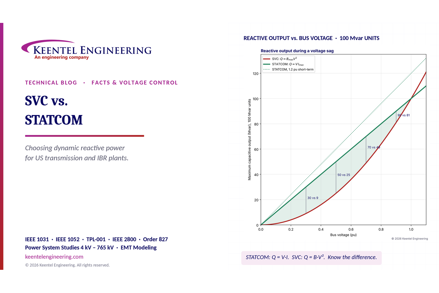
By SANDIP R PATEL
•
November 12, 2026
Compare SVC vs. STATCOM for dynamic reactive power compensation, voltage stability, weak grids, response time, harmonics and transmission system design.
By SANDIP R PATEL
•
November 11, 2026
Explore LVDC power distribution for data centers, including 380V vs 800V DC, architecture, grounding, protection, UPS, energy efficiency and safety standards.
By SANDIP R PATEL
•
November 11, 2026
Explore grid reliability vs. resilience, extreme weather planning, outage recovery, IEEE 1366 metrics, microgrids and IBR challenges with Keentel Engineering.
By SANDIP R PATEL
•
November 10, 2026
Learn NERC PRC-028-1 requirements for solar, wind and BESS, including disturbance monitoring, recording standards, deadlines and compliance steps from Keentel.
By SANDIP R PATEL
•
November 8, 2026
What does a 1 GW data center mean? Explore power capacity, PUE, GPU racks, grid interconnection and commissioning with Keentel Engineering's expert guide.