A Coordinated Electric System Interconnection Review—the utility’s deep-dive on technical and cost impacts of your project.
Challenge: Frequent false tripping using conventional electromechanical relays
Solution: SEL-487E integration with multi-terminal differential protection and dynamic inrush restraint
Result: 90% reduction in false trips, saving over $250,000 in downtime
The three operating regions you have to design to
| Device | Output vs voltage | Response | Best suited to | Main limitations |
|---|---|---|---|---|
| Mechanically switched capacitor or reactor | Proportional to voltage squared | Seconds; discrete steps; limited switching operations per day | Steady-state reactive supply, voltage profile, loss reduction | No dynamic capability; step voltage change on switching; capability collapses when most needed |
| Static var compensator | Capacitive branches proportional to voltage squared | A few cycles; continuously controllable | Continuous control where cost matters and deep voltage support is not the driver | Square-law capability loss; harmonic filters are part of the plant and interact with the network |
| STATCOM | Approximately proportional to voltage — constant current capability | One to two cycles closed loop; converter response faster still | Voltage stability margin, weak interconnections, fast disturbance recovery, flicker and unbalance compensation | Higher capital cost; converter losses; adds a converter and its control dynamics to the network |
| Synchronous condenser | Governed by machine capability and excitation | Excitation response in the hundreds of milliseconds; inherent inertial response instantaneous | System strength and inertia, short-circuit contribution, black start support | Rotating plant with maintenance and losses; slower controlled response than a converter |
| STATCOM with energy storage | Reactive as a STATCOM, plus real power within the storage rating | As STATCOM for reactive; real power limited by storage | Where a real power deficiency is part of the problem | Cost and complexity of the storage; different failure and maintenance profile |
| Service area | What we do for SST campuses | Typical deliverables |
|---|---|---|
| Grid interconnection | Site screening, large-load applications, independent studies, utility and RTO coordination in ERCOT, NYISO, PJM and other markets | Screening reports, application data packages, load flow, contingency and stability studies, study review memos |
| EMT modeling | Model requirements, vendor model review, campus aggregation, ride-through, weak-grid, control interaction and load-oscillation studies | EMT model specifications, model acceptance reports, PSCAD study reports, SCR screening |
| MV/MVDC system studies | AC and DC short-circuit, DC protection philosophy, AC protection, arc flash, grounding, insulation coordination | Study reports, protection philosophy documents, settings files, arc flash labels, interface control documents |
| Power quality | Emission requirements, frequency scans, IEEE 519-2022 compliance, filter sizing, flicker assessment | Harmonic study reports, filter specifications, monitoring plans |
| Substation and transmission design | HV/EHV substations, MV collectors, transmission lines, utility interface protection | Physical and electrical drawing packages, specifications, bills of material, protection and control design |
| NERC compliance | Registration and applicability, ride-through requirements, model validation, monitoring, compliance programs | Applicability assessments, compliance programs, evidence packages, model validation reports |
| Owner's engineer and QA/QC | SST, storage and substation specifications, design reviews, FAT and SAT plans and witnessing, multi-unit QA | Specifications, review comments, test plans, witness reports, due diligence reports |
| Onsite generation and BESS | Role definition and sizing, DC bus control architecture, fire and code compliance coordination, performance testing | Sizing studies, control architecture documents, specifications, test procedures |
Storage and generation
| Term | Meaning |
|---|---|
| AFE | Active front end. The actively switched AC/DC stage of an SST that connects to the MV grid and sets its grid behavior. |
| Aggregated model | A model in which many converters are represented by a smaller number of equivalent converters to make campus-scale simulation practical. |
| Arc flash | The release of energy from an electric arc fault, assessed as incident energy at a working distance to set PPE and safe work practices. |
| BESS | Battery energy storage system. |
| Blocking | Turning off all converter switches so the converter stops feeding current, used to limit DC faults. |
| Composite load model | A positive-sequence load model that combines several load types, such as motors, electronics and static loads. |
| DAB | Dual active bridge. An isolated DC/DC converter topology with active bridges on both sides of a high-frequency transformer. |
| DC-link | The internal DC capacitor bank between converter stages. |
| EMT | Electromagnetic transient simulation. Time-domain simulation with microsecond time steps, used to study fast converter and network behavior. |
| FAT | Factory acceptance test. |
| Grid-forming | A converter control mode that sets its own voltage and frequency reference rather than following the grid's, providing support to weak grids. |
| HIL | Hardware-in-the-loop testing, in which a real controller is tested against a real-time simulation. |
| IBR | Inverter-based resource. Generation or storage connected to the grid through power electronics. |
| Insulation coordination | Matching the insulation strength of equipment to the voltage stresses the system produces, with surge protection where needed. |
| ISC/IL | The ratio of available short-circuit current to maximum demand load current at the point of common coupling, used to set IEEE 519 limits. |
| ISOP | Input-series, output-parallel. A modular converter arrangement that shares a high input voltage across cells in series and combines their outputs in parallel. |
| Large load | A load large enough to affect transmission system reliability. Definitions vary, for example 75 MW and above under Texas SB 6, or loads above 20 MW in the federal rulemaking proposal. |
| LVDC | Low-voltage DC, such as 800 VDC or ±400 VDC rack distribution. |
| MFT | Medium-frequency transformer. The compact isolation transformer inside an SST, operating at kilohertz frequencies. |
| MMC | Modular multilevel converter. A converter built from many submodules with their own capacitors, producing a stepped multilevel waveform. |
| MVDC | Medium-voltage DC distribution, roughly 1 kV to 35 kV DC in common usage. |
| OE | Owner's engineer. An independent engineer representing the owner's technical interests. |
| PCC / POI | Point of common coupling / point of interconnection, where the campus connects to the utility system and where compliance is usually assessed. |
| PLL | Phase-locked loop. The control element that tracks grid voltage phase and frequency. |
| Positive-sequence model | A fundamental-frequency, balanced dynamic model used in PSS®E, PSLF and similar tools. |
| Ride-through | The ability to stay connected and keep operating during and after a grid disturbance within defined limits. |
| SAT | Site acceptance test. |
| SCR | Short-circuit ratio. Available short-circuit power divided by converter rating, a measure of grid strength. |
| SiC | Silicon carbide, a wide-bandgap semiconductor material that allows higher voltage, higher frequency switching. |
| SST | Solid-state transformer. A power electronic converter with a high-frequency isolation stage that replaces a 60 Hz transformer and rectifier chain. |
| Supraharmonics | Emissions in the 2 kHz to 150 kHz range, above the range covered by most harmonic limits. |
| TDD | Total demand distortion. Harmonic current distortion relative to maximum demand current, used in IEEE 519. |
| WSCR | Weighted short-circuit ratio. An SCR screen that accounts for several inverter-based plants sharing a network area. |
Links were current at publication (November 2026). Large-load rules, NERC actions and standards editions are changing quickly, so confirm current versions before relying on them.
Large-load reliability and NERC
- NERC Publishes Incident Review and Guidance on Voltage-Sensitive Large Load Integration, NERC
- Reliability Insights: Large Computational Load Risks Due to Voltage Sensitivity, NERC, September 2026
- NERC Seeks to Address Reliability Impacts from Large Load Integration, NERC presentation to FERC, April 2025
- NERC issues Level 3 Alert to address immediate risks data center loads pose to the grid, Renewable Energy World, May 2026
- NERC Voltage-Sensitive Loads, Keentel Engineering
Federal and state large-load rules
- FERC Docket RM26-4, Interconnection of Large Loads, FERC
- FERC Establishes Proceeding to Consider DOE Directive on Large Load Transmission Interconnection Rulemaking, McGuireWoods, October 2025
- Texas Senate Bill 6 Ushers in Major Overhaul of Large Load Interconnection and Grid Access Rules, Bracewell, July 2025
- Public Utility Commission of Texas Issues Proposed Rules for Large Load Interconnections, Foley & Lardner, March 2026
Solid-state transformers and DC data center power
- Solid State Transformer project, Open Compute Project
- Novel Solid-State Transformer Supports 800-V DC Power in AI Data Centers, Electronic Design
- How SSTs are Reshaping Data Center Infrastructure, Microchip Technology
Standards referenced (consult the publisher for the current edition)
Step 5 — options. Replacing or retrofitting the drives with active-front-end or 18-pulse units at about 5% THDi gives a TDD of about 1.5%. An active harmonic filter sized for the 5th and 7th could achieve a similar result at the facility level. A passive 5th-harmonic tuned filter would also work but must be checked for resonance with the utility system and with any future capacitors.
What this means for you.
The same drives can be compliant on a strong system and non-compliant on a weak one. Ask your utility for the maximum short-circuit current at the PCC early in design. If the ratio is below 50, plan for low-harmonic drives or filtering from the start; it is much cheaper than retrofitting.
9. Inverter-based resources: solar, storage and wind
Solar PV, battery energy storage and full-converter wind turbines use pulse-width-modulated inverters with output filters. They are generally low-distortion sources. IEEE Std 1547-2018 (distribution-connected resources) and IEEE Std 2800-2022 (transmission-connected resources) limit their current distortion — total rated-current distortion (TRD) of 5% with individual limits by order, measured against rated current rather than present output. In practice, quality inverters measure 1–3% at rated output.
Three cautions apply:
- Percentages rise at low output. At 10% of rated output a 2% distortion (of rated current) looks like 20% THD. Limits referenced to rated current, like TDD, avoid this trap.
- Inverters change the system's impedance. Plant collector cables, inverter output filters and capacitor banks add capacitance. They can create resonances near the 5th to 13th harmonics on the 34.5 kV collector or at a 138 kV, 230 kV or 345 kV point of interconnection, amplifying background distortion that the plant did not create.
- Background distortion matters. Inverters can absorb or amplify existing voltage distortion depending on their control design. Utilities increasingly require harmonic impedance studies for new plants, sometimes using electromagnetic transient (EMT) simulation.
Keentel's articles on harmonic resonance and on
weak-grid inverter stability cover these interactions in depth.
10. Data centers and other electronic facilities
Data centers are a special case because almost all their load is electronic. Points to check:
- UPS rectifiers. Double-conversion UPS units with IGBT rectifiers typically draw less than 5% THDi at rated load, rising at low load. Older six-pulse or 12-pulse thyristor UPS rectifiers may need input filters.
- Server and network power supplies. Modern units with active power factor correction have low 3rd harmonic. Legacy equipment does not. Measure a representative panel rather than assuming.
- 208Y/120 V and 415Y/240 V distribution. Check neutral current and transformer K-factor as in Sections 4 and 7.
- Generator operation. Test UPS and generator compatibility at the actual load level. Generator THDv can be three to four times the utility THDv for the same load.
- Cooling plant. Chiller, pump, fan and cooling distribution unit drives often contribute more low-order harmonics than the IT load. Specify low-harmonic drives where the facility is large relative to the utility source.
- Large-load interconnection. Utilities and grid operators now treat large data centers as high-impact loads. Harmonic studies and power quality monitoring are increasingly part of interconnection requirements, alongside ride-through and dynamic studies.
11. How a harmonic study is done
A harmonic study answers four questions: How much harmonic current will the facility inject? What voltage distortion will it cause? Will any resonance amplify it? What is the cheapest reliable fix? Keentel's typical workflow:
- Gather data. Single-line diagram; utility short-circuit data (maximum and minimum) at the PCC; utility background distortion if known; transformer impedances; cable lengths; capacitor banks and filters; drive, UPS and inverter data sheets with harmonic spectra.
- Measure existing conditions. For existing facilities, install class-compliant power quality meters at the PCC and key buses for at least one week, capturing 10-minute and 3-second data up to the 50th harmonic.
- Build the model. Represent sources as harmonic current injections and the network as frequency-dependent impedances, including transformer phase shifts that can cancel 5th and 7th harmonics between delta-delta and delta-wye units.
- Run a frequency scan. Plot driving-point impedance versus frequency at each important bus to find resonances, for all credible system configurations (tie breakers open/closed, capacitor steps in/out, generator versus utility).
- Run harmonic load flow. Calculate harmonic currents and voltages and compare them with IEEE 519 at the PCC and with equipment limits (IEEE 18 for capacitors, C57.110 for transformers) inside the facility.
- Design mitigation. Compare options for performance, cost, losses, footprint and future flexibility.
- Verify. Measure again after installation and document compliance with the statistical criteria.
12. Fixing harmonics: options compared
Ground Distance Protection for Transmission Lines: Application, Mho and Quadrilateral Design, Mutual Coupling and Setting Guidelines — A US Engineering Guide
November 12, 2026 | Blog
Part A — Ground Distance Protection at a Glance
Most faults on overhead transmission lines involve ground. Lightning flashes over an insulator string, a conductor sags into a tree during a hot summer afternoon, a crane boom swings into a span, a bird streamer bridges a gap, or a polymer insulator tracks after years of contamination. Utility outage statistics in the United States consistently show that single-line-to-ground faults make up roughly 70 to 80 percent of all transmission line faults, with phase-to-phase, double-line-to-ground and three-phase faults making up the rest. A protection scheme that is fast, secure and selective for ground faults is therefore not a refinement. It is the heart of transmission line protection.
For decades many US utilities protected lines against ground faults mainly with directional ground overcurrent relays (device 67N or 67G) and used distance relays (device 21) mainly for phase faults. Ground distance relays (device 21G) existed, but in the electromechanical era they required separate elements per phase, extra wiring, careful current compensation and a lot of panel space. Outside North America ground distance was standard practice much earlier. Today the picture has changed. Every modern microprocessor-based line relay sold into the US market includes ground mho and ground quadrilateral elements as standard features. Turning them on takes a few settings rather than a new panel. That convenience is exactly why ground distance deserves careful engineering: it is easy to enable, and it is just as easy to enable badly.
Ground distance elements behave very differently from phase distance elements. They depend on a zero-sequence compensation factor that is only as good as the line data behind it. They are influenced by zero-sequence mutual coupling from parallel circuits that may share a right-of-way for only part of the route. They respond to fault resistance, arc resistance and tower footing resistance that phase faults rarely involve. They can be fooled by a tapped wye-grounded transformer, an in-line autotransformer, a series capacitor, an underground cable whose ground return path changes with the fault location, or an inverter-based resource that supplies little or no negative-sequence current. Each of these effects can make a ground distance zone overreach and trip for an external fault, or underreach and fail to trip for an internal fault.
This guide is Keentel Engineering's full-depth treatment of how to apply and set ground distance elements on US transmission lines from 69 kV through 765 kV. It covers element design, the mho and quadrilateral characteristics and their polarizing quantities, the major application challenges, and a complete set of setting guidelines with worked examples. It is written for practicing protection engineers, but it also explains, in plain language, what owners, developers and compliance managers need to know to judge whether their ground distance settings are sound.
In plain terms: a ground distance relay estimates how far away a ground fault is by dividing a voltage by a specially compensated current. If the compensation is wrong, if a parallel line adds an unseen voltage, if the fault has resistance, or if the instrument transformers distort the signals, the estimate is wrong. Good settings come from understanding each of those errors and leaving enough margin for them, and from verifying the result with a fault study rather than with the line impedance alone.
Who this guide is for
This guide is written for several audiences, and each can read it differently.
- Protection and control engineers at utilities, transmission owners, generator owners and consulting firms who calculate, review or test ground distance settings. Part B and the worked examples are written for you.
- Interconnection customers and developers of solar, wind, battery storage and large load facilities such as data centers, whose generator tie lines and interconnection substations need line protection that coordinates with the host utility. The sections on weak sources, inverter-based resources and tapped transformers are especially relevant.
- Compliance managers responsible for NERC PRC standards, who need to understand how ground distance settings relate to misoperation analysis, protection system maintenance and coordination studies.
- Asset managers and planners who are adding parallel circuits, series compensation, underground cable sections or new taps, and who need to know which existing relay settings those projects will disturb.
How to read this guide
Part A gives the big picture, the key terms, the headline setting rules and a review of common statements about ground distance that need correction or qualification. Part B is the engineering guide. It works through element design, each application challenge and the setting process, with equations, tables and worked examples. Each major section ends with a short note on how Keentel Engineering helps clients with that topic. Part C presents three anonymous US case studies drawn from the kinds of problems we see in practice. Part D is a 30-question technical FAQ. The guide closes with Keentel's services, references and contact information.
All examples use 60 Hz US system conditions, US transmission voltages and US units. Line impedances are given in ohms per mile unless otherwise stated. Impedances are primary ohms unless marked secondary. Every worked example was checked with an independent sequence-network calculation, and the numbers in this guide reproduce those results.
Why ground distance matters more now
Several trends are pushing ground distance elements from optional to essential on the US grid.
- Microprocessor relays made it free to enable. Ground mho and quadrilateral zones are already in the relay. The cost question has disappeared, and the engineering question has taken its place.
- Ground overcurrent coordination is getting harder. As networks become more meshed and more transformers are added, zero-sequence current distributes in ways that make time-overcurrent coordination slow and fragile. Ground distance zones provide a defined reach that does not depend on fault current magnitude in the same way.
- Inverter-based resources change fault signatures. Solar, wind and battery plants interconnected through wye-grounded/delta step-up transformers are strong zero-sequence sources but often weak positive- and negative-sequence sources. Ground distance and negative-sequence elements behave differently in these systems, and settings that worked with synchronous generation may need review.
- Rights-of-way are crowded. New circuits are increasingly built on existing corridors, on double-circuit towers or alongside lines at other voltages. Each new parallel path adds zero-sequence mutual coupling that changes what existing ground distance relays measure.
- NERC expectations are explicit. PRC-004 requires misoperation identification and corrective action plans. PRC-027 requires a coordination process for new and changed protection systems. A ground distance misoperation caused by an unmodeled mutual impedance is a reportable event with a corrective action plan, not just an engineering curiosity.
- Large loads are arriving fast. Hyperscale data center campuses connected at 138 kV, 230 kV and 345 kV add new substations, new taps and new transformers to existing lines, often on aggressive schedules. Each one changes the zero-sequence network that existing ground distance relays see.
Key terms used in this guide
The following terms appear throughout the guide.
| Term | Meaning in this guide |
|---|---|
| Ground distance element (21G) | An impedance-measuring element that responds to phase-to-ground faults using a phase voltage and a compensated phase current. |
| Fault loop | The combination of voltage and current a distance element measures: three ground loops (AG, BG, CG) and three phase loops (AB, BC, CA). |
| Apparent impedance | The impedance a relay calculates during the fault from measured loop voltage and loop current; it equals the true fault impedance only under ideal conditions. |
| Zero-sequence compensation factor (k0) | The complex factor that relates residual current to the ground loop impedance, correcting zero-sequence line impedance; k0 = (Z0 − Z1)/(3Z1). |
| Mutual compensation factor (k0M) | An optional factor that adds the parallel line residual current to the loop current to correct zero-sequence mutual coupling. |
| Mho characteristic | A circular operating characteristic on the R-X plane, defined by a phase comparator between an operating and a polarizing quantity. |
| Quadrilateral characteristic | A four-sided characteristic made of a reactance line, two resistive blinders and a directional line. |
| Polarizing quantity | The reference phasor a comparator uses; for mho elements usually positive-sequence memory voltage, for quadrilateral reactance lines often negative- or zero-sequence current. |
| Homogeneity | The condition where source and line impedance angles are equal so fault current at the fault and current at the relay are in phase. |
| TIL (non-homogeneity correction) | An angular adjustment to the quadrilateral reactance line that accommodates for non-homogeneity when fault resistance is present. |
| SIR | Source-to-line impedance ratio; the source impedance behind the relay divided by the protected line impedance. |
| Zone 1 | An instantaneous zone set at high, without intentional delay, typically 80–85 percent of the line. |
| Zone 2 | An overreaching zone used for forward backup and as part of pilot schemes. |
| Zone 3 | A farther zone, used for remote backup in three-distance schemes or as a reverse-looking blocking zone in pilot schemes. |
| POTT, DCB, DCUB | Permissive overreaching transfer trip, directional comparison blocking and directional comparison unblocking pilot schemes. |
| CVT | Coupling-capacitor voltage transformer, common at 115 kV and above. |
| SPT | Single-pole tripping, in which only the faulted phase is opened for a single-line-to-ground fault. |
| IBR | Inverter-based resource such as a solar, wind or battery plant. |
The one equation every ground distance setting depends on
A ground distance element must measure the positive-sequence impedance to a ground fault, because that is the quantity the reach is set in. For a bolted A-phase-to-ground fault at a fraction m of the line length, the phase voltage at the relay is the sum of positive-, negative- and zero-sequence voltage drops along the line. Writing the line drop in terms of the relay's phase current and residual current gives the classic result:
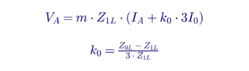
The relay therefore divides the A-phase voltage by the compensated loop current, IA + k0·3I0, and the result is m·Z1L, which is directly proportional to the distance to the fault. That single equation explains almost every ground distance problem in this guide. Anything that adds a voltage the equation does not include, such as fault resistance, mutual coupling or a series capacitor, or anything that makes the line Z0 different from the value used to compute k0, such as a cable sheath return path or a tapped grounded transformer, produces an error in the measured distance.
Mho versus quadrilateral at a glance
| Attribute | Ground mho | Ground quadrilateral |
|---|---|---|
| Shape on R-X plane | Circle through origin (self-polarized), expanding with memory polarization | Four-sided polygon with independent reactive and resistive reach |
| Fault resistance coverage | Moderate; depends on reach, source strength and memory decay; least near the reach point | Set directly by the resistive blinders; same coverage along the whole line |
| Security under heavy load | Inherently good; the circle stays narrow near the load region | Requires the resistive blinder to be set clear of load; load encroachment logic may be needed |
| Effect of non-homogeneity with fault resistance | Present but limited by the shape of the circle | Significant; requires tilt or sequence-current polarizing of the reactance line |
| Best applications | Long lines, heavily loaded lines, pilot schemes, single-pole tripping, cables | Short lines with strong sources, step-distance backup without pilot channels, high footing resistance areas |
| Setting effort | Lower; reach and angle | Higher; reactive reach, resistive reach, tilt, polarizing choice, directional angle |
| Coordination | Reach expansion differs by relay design | Resistive reach definitions differ by relay design; coordination must be checked with resistive faults |
Headline setting rules
The following table summarizes the setting rules developed in Part B. Each rule has exceptions, which Part B explains.
| Zone or setting | Typical starting point | Key checks |
|---|---|---|
| Zone 1 reactive reach | 80 to 85 percent of the lowest apparent impedance for a remote-bus ground fault | Mutual coupling with parallel line out and grounded; tapped transformers; CVT transients; high SIR; series capacitors |
| Zone 2 reactive reach | At least 120 percent of the highest apparent impedance for a remote-bus ground fault; often 125 to 150 percent | Infeed; mutual coupling with parallel line in service; coordination with Zone 1 of the shortest adjacent line |
| Zone 2 time delay | 15 to 30 cycles in step-distance schemes | Breaker failure timing; adjacent line Zone 1 and breaker clearing time |
| Pilot overreaching zone | Often around 150 to 200 percent of the line | Reverse blocking zone must overreach the remote forward zone |
| Reverse blocking zone | Set to cover everything the remote overreaching zone can see behind the local bus | Check with bolted and resistive faults, including current reversal |
| Zone 3 (step distance) | Remote backup, limited by load and by system topology | Load encroachment, power swing and loadability review |
| Quadrilateral resistive reach | Between the arc resistance requirement and a margin below minimum load impedance at 0.85 pu voltage | Steady-state angle error limit; non-homogeneity tilt; relay-specific definition of resistive reach |
| k0 | (Z0L − Z1L)/(3·Z1L) from validated line constants | Relay-specific format (magnitude and angle, or separate RE/RL and XE/XL) |
| Ground current supervision | Below the minimum 3I0 for a remote-bus fault with a weak source | Must remain above the standing unbalance and CT error |
A review of common statements about ground distance
Industry literature on ground distance is generally sound, but several statements are often repeated without the conditions that make them true. In preparing this guide Keentel Engineering reviewed widely circulated guidance and checked the key claims against first principles and independent calculations. The table below summarizes what holds and what needs qualification.
| Common statement | Keentel assessment | What to do instead |
|---|---|---|
| "Mutual coupling makes the line look longer." | True only when the parallel line is in service and its zero-sequence current flows in the same direction. With the parallel line out of service and grounded at both ends, the line looks shorter, and Zone 1 can overreach the remote bus. In our 34.5 kV double-circuit example, the measured reactance for a remote-bus fault ranges from 0.83 to 1.29 times the true value depending on the parallel line state. | Set Zone 1 from the lowest apparent impedance across all credible parallel line states and set overreaching zones from the highest. |
| "Maximum quadrilateral resistive reach is about five times the reactive reach." | This ratio comes from one example: a Zone 1 reach of 80 percent and a total angular error of 3 degrees. With an 85 percent reach and the same error, the limit is about 3.4 times. With 5 degrees of error it drops to about 2 times. | Calculate the limit for your actual Zone 1 margin and instrument transformer accuracy using the appropriate resistive-reach formula. |
| "The Blackburn arc formula is the most restrictive." | It depends on fault current. At about 1,000 A the Warrington formula gives the highest arc resistance; at 5,000 A and above the Blackburn formula gives the highest. All three common formulas agree only within a factor of about two to three. | Use the formula that is most conservative at the actual fault-current range, and add arc stretch and structure footing resistance where there is no shield wire. |
| "Zone 1 is set to 80 to 85 percent of the line." | A good starting point for a homogeneous two-terminal overhead line. It is not adequate where mutual coupling, a tapped grounded transformer, a series capacitor or a high SIR is present. | Base Zone 1 on the lowest apparent impedance from a fault study, not on the positive-sequence line impedance alone. |
| "CT saturation affects dependability, not security." | Largely true for distance elements: saturation tends to make the relay underreach. It can still affect security through false residual current during transformer energization and through phase-angle shift that disturbs directional decisions. | Size CTs for the overreaching pilot zone and verify residual current behavior during inrush. |
| "Mho elements are inherently secure under load." | True for elements set along the line angle with ordinary reach, but a long Zone 3 or a heavily expanded memory-polarized mho element can still approach load. | Check every zone against the load impedance at 0.85 pu voltage and the applicable PRC-023 loading criteria for phase elements. |
| "Disable Zone 1 when SIR exceeds a fixed number." | Fixed thresholds such as SIR 20 or 30 depend strongly on CVT design and relay filtering. A threshold appropriate for one relay and one CVT type may be unnecessarily restrictive or unsafe for another. | Calculate the SIR under N-1 conditions, find the relay maker's published CVT transient performance and consider pilot schemes for short lines. |
| "A ground backup zone should be delayed at least 1.5 seconds on single-pole-tripped parallel lines." | The required delay depends on the single-pole dead time used on the parallel line. Systems with shorter dead times need less delay; longer dead times need more. | Coordinate the extended ground zone delay with the actual single-pole reclose dead time plus margin, or block the element during the open-pole interval. |
Eight findings for decision makers
For readers who will not go further than Part A, these are the most important findings in this guide.
1. Ground distance settings cannot be calculated from the line impedance alone. On any line with a parallel circuit, a tapped grounded transformer, an autotransformer, a series capacitor or a cable section, the apparent impedance for a remote-bus fault differs from the line impedance, sometimes by 20 to 30 percent. A fault study with mutual impedances modeled is mandatory.
2. The worst case for Zone 1 is often the parallel line out of service and grounded. That maintenance condition can make the line look shorter by close to 20 percent. A Zone 1 set to 85 percent of the line impedance can then reach past the remote bus.
3. Fault resistance coverage is the main reason to use quadrilateral elements. Where step-distance backup must cover resistive faults on short, strongly sourced lines, quadrilateral elements outperform mho elements. Where a pilot scheme exists, mho elements usually provide comparable coverage with less setting risk.
4. Quadrilateral elements need non-homogeneity correction. On a non-homogeneous system, fault resistance shifts the measured reactance. In our 230 kV example, a 30-ohm fault at the Zone 1 reach point appears 14 percent closer than it is when the local source angle is low. A small reactance tilt eliminates that error.
5. Ground overcurrent and pilot schemes still matter. No distance element covers as much fault resistance as a sensitive directional ground overcurrent element or a line current differential scheme. Ground distance complements these functions rather than replacing them.
6. Underground cables challenge ground distance. The zero-sequence impedance of a cable depends on how the fault current returns through sheaths, earth and nearby metallic paths. A k0 chosen for one return path can make the element underreach by a factor of two or more for a different path. Line current differential is usually preferred for cables.
7. Inverter-based resources change the rules. Weak and unconventional negative-sequence current from inverters can disturb fault-type selection and negative-sequence-polarized elements. Ground distance at IBR interconnections must be checked with realistic inverter models and the IEEE 2800 response of the plant.
8.
Documentation and testing protect you during audits and after events. A setting file supported by a fault study, a written philosophy and a test record is the best evidence for PRC-004 misoperation analysis and PRC-027 coordination reviews.
Part B — Engineering Guide: Applying and Setting Ground Distance Elements
1. Distance protection fundamentals
The balance-beam picture
The simplest way to picture a distance relay is a balance beam. Voltage pulls on one side and acts as a restraining force. Current pulls on the other side and acts as an operating force. During normal operation a 115 kV transmission line relay sees a secondary phase voltage near 66.4 V and a load current of a few amperes secondary, and the beam stays on the restraint side. When a fault occurs, the voltage at the relay collapses and the current rises. If the ratio of voltage to current falls below the relay's setting, the beam tips, the trip contact closes and the breaker opens.
The ratio of voltage to current is an impedance, so the relay is really measuring impedance. Because the impedance of a transmission line is proportional to its length, measuring impedance is equivalent to measuring distance. That is the reason distance relays are attractive: their reach is defined by the line itself rather than by the fault current, which changes with system conditions.
Electromechanical relays implemented this balance with induction cups and cylinder units. Static relays used analog comparators. Microprocessor relays sample the voltages and currents, filter them to extract the 60 Hz phasors, and evaluate the comparator equations in software many times per cycle. The principles are unchanged, but the modern relay can implement any characteristic shape and polarizing method, which is both a strength and a source of variation between relay designs.
Reach, line angle and the R-X plane
Distance settings are expressed on the complex impedance plane, called the R-X plane, with resistance on the horizontal axis and reactance on the vertical axis. A transmission line appears as a straight line from the origin at the line impedance angle. For overhead transmission lines in the US this angle is typically 75 to 88 degrees: about 70 to 80 degrees at 69 kV, 80 to 85 degrees at 115 to 230 kV, and 85 to 88 degrees at 345 kV and above with bundled conductors.
The reach of a distance zone, ZR, is a complex impedance with magnitude and angle. It is usually set at or near the line angle. Faults on the line plot along the line impedance, and fault resistance moves the measured point to the right. Load plots far to the right of the line, near the resistive axis. Power swings travel across the plane along paths determined by the source impedances. Good settings keep the zones around the line and the fault resistance region while staying clear of load and stable swings.
The six fault loops
A three-phase line has six possible fault loops. A distance relay evaluates each one with a specific combination of voltage and current.
| Distance loop | Loop voltage | Loop current | Apparent impedance |
|---|---|---|---|
| AG | VA | IA + k0·3I0 | VA / (IA + k0·3I0) |
| BG | VB | IB + k0·3I0 | VB / (IB + k0·3I0) |
| CG | VC | IC + k0·3I0 | VC / (IC + k0·3I0) |
| AB | VA − VB | IA − IB | (VA − VB) / (IA − IB) |
| BC | VB − VC | IB − IC | (VB − VC) / (IB − IC) |
| CA | VC − VA | IC − IA | (VC − VA) / (IC − IA) |
The phase loops measure positive-sequence impedance naturally, because the zero-sequence components cancel in the phase-to-phase differences. The ground loops need the k0·3I0 term to compensate for the different zero-sequence impedance of the line. This is why ground distance elements are more sensitive to errors in line data than phase distance elements.
Deriving the ground loop equation
Consider a bolted A-phase-to-ground fault at a per-unit distance m from the relay on a line with positive-, negative- and zero-sequence impedances Z1L, Z2L = Z1L and Z0L. The sequence voltages at the relay exceed those at the fault by the sequence voltage drops along the faulted portion of the line:

At a bolted A-phase fault the A-phase voltage at the fault is zero, so V1F + V2F + V0F = 0. Adding the three equations

Writing the bracket in terms of residual current 3I0 gives the compensated loop current and the definition of k0:
This result holds regardless of the source impedances, the load or the fault current distribution, as long as the fault is bolted, the line is homogeneous, there is no mutual coupling and no other source of zero-sequence current enters the line between the relay and the fault. Every application challenge in this guide is a violation of one of those assumptions.
Different k0 formats used by relays
Relay designs express zero-sequence compensation in several ways. Engineers must convert carefully, because using the wrong format is a common source of large reach errors.
| Format | Definition | Notes |
|---|---|---|
| Complex k0 (magnitude and angle) | k0 = (Z0L − Z1L)/(3·Z1L) | The most common modern format; angle is usually small and negative for overhead lines |
| Separate resistive and reactive factors | RE/RL = (R0L − R1L)/(3·R1L) and XE/XL = (X0L − X1L)/(3·X1L) | Used by some relay families; RE/RL and XE/XL can differ greatly because R0/R1 is much larger than X0/X1 |
| Z0/Z1 ratio | Z0L/Z1L magnitude and angle | Some relays accept the ratio and compute k0 internally |
| Residual compensation without the factor of 3 | kN = (Z0L − Z1L)/Z1L applied to I0 | Mathematically equivalent when the relay uses I0 rather than 3I0 |
| Ground return impedance | ZE = (Z0L − Z1L)/3 in ohms | Some relays ask for the ground return impedance itself |

Step 2. Complex k0. The ratio Z0L/Z1L is 3.11∠−3.3°. Therefore:

Step 3. Separate resistive and reactive factors.

Note how different the two factors are. An engineer who enters 0.70 into both fields of a relay that uses the separate format will under-compensate the resistive part by a factor of 1.7, which shifts the measured fault impedance and alters the resistive coverage near the reach point.
Step 4. Secondary conversion. With 2000:5 CTs (ratio 400) and 230 kV to 115 V VTs (ratio 2000), the secondary-to-primary factor is 400/2000 = 0.2:

The starting reach values are summarized below. They are only starting points: Section 14 shows how they must be adjusted with a fault study.
| Zone | Percent of Z1L | Primary ohms | Secondary ohms |
|---|---|---|---|
| Zone 1 | 80% | 31.46 | 6.29 |
| Zone 1 | 85% | 33.42 | 6.68 |
| Zone 2 | 120% | 47.18 | 9.44 |
| Zone 2 | 125% | 49.15 | 9.83 |
| Pilot overreach | 150% | 58.98 | 11.80 |
| Pilot overreach | 200% | 78.64 | 15.73 |
Where line constants come from, and why they are uncertain
Positive-sequence impedance can be calculated accurately from conductor and spacing data, and it rarely differs from measured values by more than a few percent. Zero-sequence impedance is far less certain. It depends on earth resistivity, which varies with season, moisture and geology; on shield wire type and grounding; on the tower footing resistances; and on any nearby metallic paths such as pipelines and railroads. A 2:1 change in earth resistivity changes Z0 by only a few percent, but errors in shield wire modeling, missing segments of a route, or mixed construction can produce errors of 10 to 20 percent in Z0. That uncertainty flows straight into k0.
Keentel's practice is to build line models from as-built route data, segment by segment, including every change of structure type, conductor, shield wire and parallel circuit, and to compare calculated impedances with field measurements where line impedance testing is available. When measurements are not available, we add margin to Zone 1 rather than relying on a single theoretical Z0.
How Keentel Engineering helps here: We calculate line constants from as-built route data, including shield wires, segment changes and every parallel circuit that shares the corridor, and we convert them into the exact k0 format each relay requires. Our setting files show the calculation trail from tower geometry to secondary ohms so that reviewers and auditors can follow every number.
2. Ground mho element design
The mho characteristic
The mho characteristic is a circle on the R-X plane whose diameter is the reach impedance ZR. A self-polarized mho circle passes through the origin and through the reach point. If the measured impedance plots inside the circle, the element operates. If it plots outside, the element restrains.
The circular shape is not drawn directly. It emerges from a phase comparator. The relay forms two phasors: an operating quantity and a polarizing quantity. For a ground loop the current I is the compensated loop current IA + k0·3I0, and V is the loop voltage VA.

The element operates when the angle between the operating and polarizing quantities is 90 degrees or less:

When the polarizing quantity is the loop voltage V itself, the boundary condition, an angle of exactly 90 degrees between I·ZR − V and V, describes a circle with I·ZR as its diameter. Dividing every phasor by the current I translates the voltage-plane picture into the impedance plane, and the circle has ZR as its diameter. Inside the circle the angle is less than 90 degrees and the element operates. Outside it is greater than 90 degrees and the element restrains.
Microprocessor relays often implement the same comparison as a torque-like product. The element operates when the real part of the operating phasor multiplied by the conjugate of the polarizing phasor is positive:
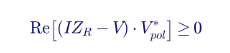
Many designs solve this expression for the reach at which the element would just operate and compare that value with the setting. The mathematics is equivalent; the implementation choice affects speed, filtering and the behavior at the boundary.
Why self-polarization is not enough
A self-polarized mho element has a serious limitation. For a bolted fault directly in front of the relay, the loop voltage collapses to nearly zero. With no voltage, there is no polarizing reference, and the element cannot determine direction or operate reliably. In practice the element may fail to trip for a close-in fault, the very fault that most needs fast clearing. It may also operate for a close-in reverse fault, because noise and filter transients dominate the comparison when the voltage is near zero.
Relay designers solved this problem with two techniques that are now universal: cross-polarization and memory polarization.
Cross-polarization
Cross-polarization uses the voltages of the unfaulted phases to create the polarizing reference. For an A-phase-to-ground fault the B-C voltage remains healthy. Rotated by 90 degrees, it is in phase with the prefault A-phase voltage:
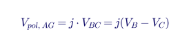
Cross-polarization works well for ground faults, because the unfaulted phases keep their voltage. It does not work for a three-phase fault at the relay location, where all three voltages collapse. That gap is filled by memory.
Memory polarization with positive-sequence voltage
Modern relays commonly polarize ground mho elements with positive-sequence voltage memory. The relay continuously stores the prefault positive-sequence voltage, rotates it to the appropriate phase reference, and uses it as the polarizing quantity for a period after the fault begins. The memory decays with a time constant chosen by the relay designer, typically a few cycles to several tens of cycles, and many designs blend memory and present positive-sequence voltage so the element remains polarized for sustained faults.
| Element | Operating quantity | Self-polarized reference | Cross-polarized reference | Positive-sequence memory reference |
|---|---|---|---|---|
| AG | (IA + k0·3I0)·ZR − VA | VA | j·VBC | V1 memory, A-phase reference |
| BG | (IB + k0·3I0)·ZR − VB | VB | j·VCA | V1 memory rotated by 240° |
| CG | (IC + k0·3I0)·ZR − VC | VC | j·VAB | V1 memory rotated by 120° |
Positive-sequence voltage is attractive because it contains contributions from all three phases, it is always present for unbalanced faults, and it is retained in memory for balanced close-in faults.
Mho expansion: why memory polarization adds resistive coverage
Memory polarization does more than fix close-in faults. It changes the shape of the characteristic for forward faults. Because the prefault voltage at the relay can be written as the fault voltage plus the drop across the local source impedance, the polarizing quantity behaves as if the relay were measuring from a point behind the source. The resulting forward characteristic is still a circle, but its diameter now extends from the reach point ZR back to −ZS, where ZS is the local source impedance:

Three properties of this expanded circle are important for settings:
- The reach point does not move. The expanded circle still passes through ZR, so memory polarization does not cause overreach along the line angle.
- The expansion grows with source impedance. A weak source, with a large ZS, produces a large expansion and good resistive coverage. A strong source produces little expansion. Paradoxically, the relay gets the least resistive coverage on short lines with strong sources, where fault currents are high and arc resistance is lowest, and the most on weak systems.
- The expansion is a forward-fault phenomenon. For reverse faults the same polarizing quantity shifts the circle away from the origin into the first quadrant, which makes the element secure for reverse faults.
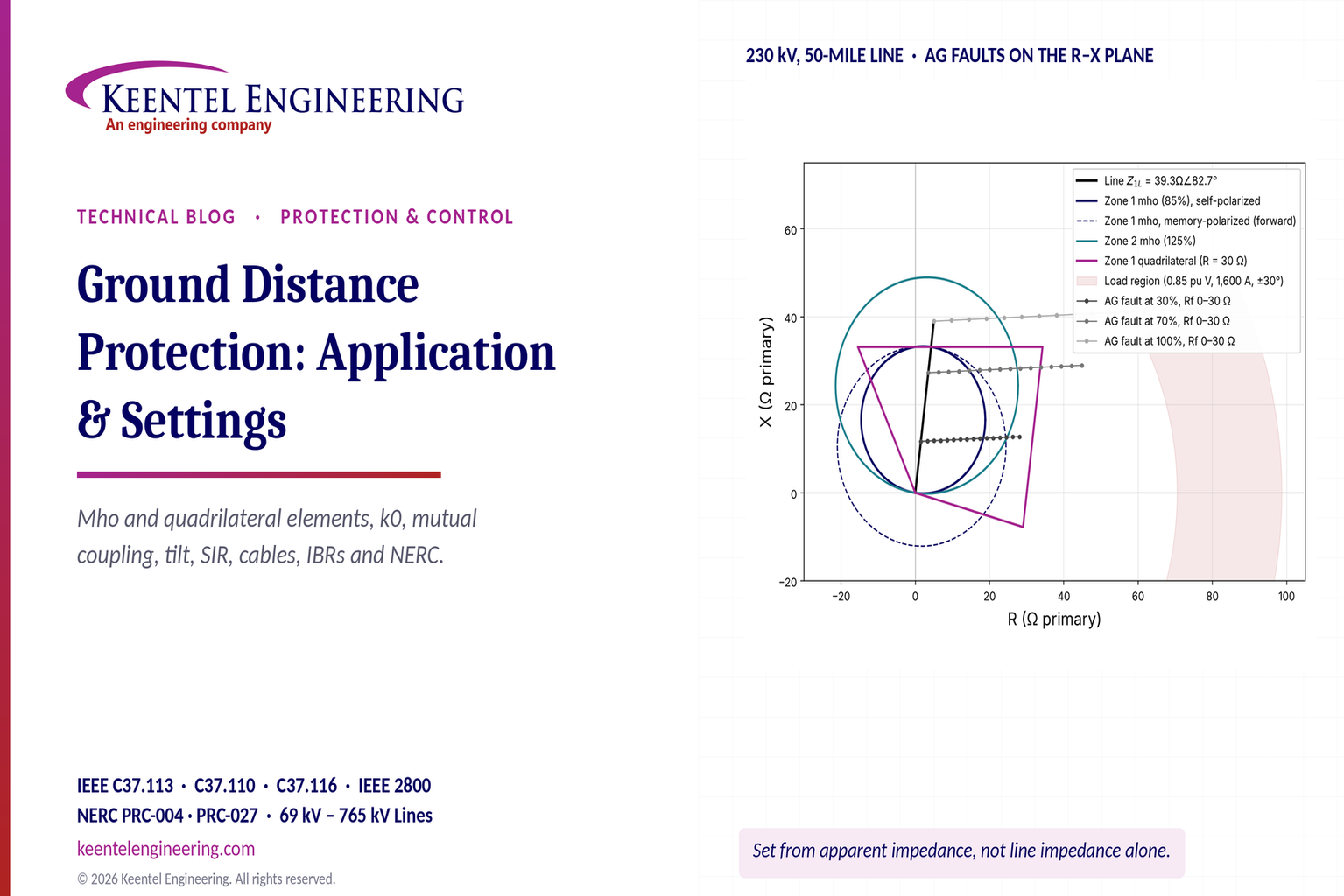
In the R-X diagram of this guide, the dashed circle shows the forward expanded Zone 1 characteristic for the 230 kV example with a 12-ohm local source. It reaches the same point on the line but covers substantially more resistance near the relay.
Offset mho and its uses
Some applications use an offset mho characteristic, a circle that includes a small region behind the relay. Offset characteristics provide dependable operation for close-in three-phase faults without relying on memory, and they are commonly used for switch-onto-fault logic and for reverse-looking zones in some pilot scheme designs. Because an offset zone includes the origin, it is not directional and must be time-delayed or supervised when used for tripping.
Resistive coverage of a mho element
The resistive coverage of a self-polarized mho element at a fault location m is the horizontal width of the circle at that point. For a fault close to the reach point the coverage approaches zero. For a fault at the midpoint of the reach it is greatest. With a reach of magnitude r at angle θ, and a fault whose bolted impedance d = m·|ZL| lies along the same angle, the largest purely resistive addition R that keeps the measured point inside the circle is:

For the 230 kV example with an 85 percent Zone 1 reach (r = 33.4 ohms at 82.7 degrees), a fault at 30 percent of the line (d = 11.8 ohms) can tolerate about 17 ohms of apparent resistance, a fault at 70 percent (d = 27.5 ohms) only about 11 ohms, and a fault at 84 percent (d = 33 ohms) about 2 ohms. Remember that the apparent resistance is the fault resistance multiplied by the infeed ratio, which is usually greater than one, so the actual fault resistance covered is smaller still. The practical conclusion is simpler: a mho element offers most of its resistive coverage in the first half of its reach, and very little near its reach point. Memory polarization improves that coverage, especially on weak systems. Section 4 compares these coverages with those of a quadrilateral element.
What the mho element does well
The mho element has survived nearly a century of relay technology because it combines three qualities in one simple comparison:
- It is directional by construction. The characteristic passes through or near the origin, so a separate directional element is not needed for basic operation.
- It is secure against load. The circle is narrow in the resistive direction near the reach point, which keeps it away from the load region on long lines.
- It is predictable for coordination. The reach along the line angle is unaffected by polarization, and the expansion is a well-understood function of the source impedance.
How Keentel Engineering helps here: We model the actual polarizing method and memory behavior of the installed relay, rather than a generic circle, when we evaluate fault resistance coverage and coordination. Our studies show clients where their mho elements provide adequate resistive coverage and where a quadrilateral element, a pilot scheme or ground overcurrent backup is needed.
3. Ground quadrilateral element design
Why a quadrilateral?
Ground faults often involve resistance. An arc across an insulator string has a resistance of a few ohms that grows as wind stretches the arc. A tree contact can present tens of ohms. A conductor lying on dry ground or sand can present hundreds. On lines without shield wires, the tower footing resistance appears in series with the arc. A mho element sized to reach 85 percent of a short line has a very small circle and covers little of that resistance. A quadrilateral element solves the problem by separating the two dimensions of the characteristic: the reactive reach is set by the line, and the resistive reach is set by the fault resistance to be covered and the load to be avoided.
The four lines
A ground quadrilateral characteristic is the logical AND of four straight-line boundaries on the R-X plane:
- The reactance line (top). Sets the reach along the line. It is horizontal in the basic form, and it can be tilted to correct for non-homogeneity.
- The right resistive blinder. Parallel to the line impedance angle, offset to the right by the resistive reach setting. It limits coverage in the load direction.
- The left resistive blinder. Parallel to the line or set at a fixed angle in the second quadrant, offset to the left. It limits reverse-direction and power swing coverage.
- The directional line (bottom). Passes through or near the origin, usually tilted a few degrees below the resistive axis. It separates forward from reverse faults and is often supervised by a separate negative-sequence or zero-sequence directional element.
A fault is inside the zone only if it is above the directional line, below the reactance line, to the left of the right blinder and to the right of the left blinder. Each boundary is implemented with its own phase comparator, and the zone output requires all four comparators to agree. The operating time of the element is therefore the longest of the four decision times, which is one reason some quadrilateral implementations are slightly slower than mho elements for faults near the zone boundary.
Each boundary is a phase comparison
Every straight-line boundary can be written as a comparison between two phasors, call them signal A and signal B, in which the boundary is crossed when the angle between them passes through 0 or 180 degrees. For the reactance line, a common form is:
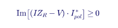
Here I is the compensated loop current, ZR is the reactive reach set along the line angle, V is the loop voltage, and Ipol is the polarizing current, the quantity that defines the direction of the reactance line. If Ipol is the loop current itself, the boundary is a straight line parallel to the resistive axis passing through ZR, a pure reactance element. If Ipol is the negative-sequence or zero-sequence current, the boundary tilts according to the phase difference between that current and the loop current.
The resistive blinder uses a similar comparison with the resistive reach RR rotated to the line angle, and the directional line compares the loop current with a voltage reference. Relay instruction manuals describe the exact signals for each boundary, and they vary between designs. What matters for settings is that the polarizing choice for the reactance line determines how the element responds to fault resistance on a non-homogeneous system.
How fault resistance moves the measured impedance
For a single-line-to-ground fault at distance m with fault resistance Rf, the relay's loop voltage includes the drop across Rf, which carries the total fault current from both line ends, not just the relay's current:
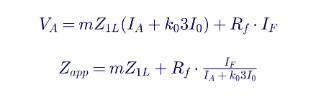
The second term is the apparent fault resistance. Its magnitude is larger than Rf when the remote end contributes current, because IF includes the remote infeed. Its angle equals the angle of IF relative to the relay's loop current. If the two currents are in phase, the fault resistance adds a purely resistive component and the measured reactance is unaffected. If IF leads the relay current, the apparent resistance rotates downward and the relay sees the fault closer than it is, which is overreach. If IF lags, the apparent resistance rotates upward and the relay underreaches.
Two conditions make the currents differ in phase:
- Prefault load. At the sending end of an exporting line the local source voltage leads the remote source voltage. The remote contribution to the fault lags the local one, and the total fault current tends to lead the relay's measured current, so the sending-end relay overreaches. The receiving end underreaches.
- Non-homogeneity. If the source and line impedance angles differ, the current distribution factor at the relay is complex, and the relay current is phase shifted from the total fault current even with no load.
Worked Example 2 apparent impedance for a resistive ground fault
Return to the 230 kV, 50-mile line of Worked Example 1, with Z1L = 39.32∠82.7° ohms and k0 = 0.70∠−4.9°. The local source (Bus S) has Z1S = 12∠86° and Z0S = 30∠80° ohms. The remote source (Bus R) has Z1R = 20∠84° and Z0R = 45∠78° ohms. Both sources are at 1.0 per unit (132.8 kV line-to-neutral) with no load. An A-phase-to-ground fault is applied at 70 percent of the line from Bus S.
Solving the sequence networks gives the following results at the Bus S relay:
| Fault resistance | Total fault current | Relay IA | Relay 3I0 | Relay voltage | Apparent impedance | Measured X / true X |
|---|---|---|---|---|---|---|
| 0 ohms | 4,800 A | 2,090 A | 1,988 A | 0.72 pu | 27.52∠62.7° (3.50 + j27.30) | 1.000 |
| 10 ohms | 4,303 A | 1,873 A | 1,782 A | 0.77 pu | 32.78∠58.2° (17.27 + j27.86) | 1.020 |
| 20 ohms | 3,629 A | 1,580 A | 1,503 A | 0.83 pu | 42.08∠42.5° (31.04 + j28.41) | 1.041 |
Several lessons come out of this table.
First, the apparent resistance is larger than the fault resistance. A 10-ohm fault adds 13.8 ohms of apparent resistance, a multiplication of about 1.38, because the remote end supplies part of the fault current that flows through Rf. The multiplication factor equals the ratio of total fault current to compensated loop current at the relay. For a fault close to a strong remote terminal, this factor can exceed 3 or 4.
Second, even with no load, the measured reactance rises slightly with fault resistance. The sources here are nearly but not perfectly homogeneous, so a 20-ohm fault makes the relay underreach by about 4 percent.
Third, the mho element runs out of coverage quickly. Using the expression for mho resistive coverage from Section 2, the Zone 1 mho at 85 percent tolerates about 11 ohms of apparent resistance at 70 percent of the line. The 10-ohm fault produces 13.8 ohms of apparent resistance plus the line resistance, so a self-polarized Zone 1 mho would not operate. A Zone 1 quadrilateral with a 30-ohm resistive reach would operate for both the 10-ohm and 20-ohm faults. Memory polarization would expand the mho circle and recover part of that coverage.
Fourth, load changes the picture. Repeating the remote-bus fault with 10 ohms of fault resistance and a 15-degree prefault angle across the system gives these results:
| Condition | Apparent impedance | Measured X / true X | Effect |
|---|---|---|---|
| No load | 49.15∠54.4° | 1.025 | Slight underreach |
| Bus S exporting (+15°) | 44.52∠53.7° | 0.920 | 8 percent overreach |
| Bus S importing (−15°) | 54.30∠56.8° | 1.163 | 16 percent underreach |
An 8 percent overreach at the exporting end, for a fault at the remote bus with only 10 ohms of resistance, would be enough to defeat a Zone 1 reactance reach set at 90 percent. This is the classic reason why quadrilateral reactance lines need either a tilt or a polarizing quantity that is not affected by load.
Polarizing the reactance line
Relay designs use three main polarizing currents for the ground quadrilateral reactance line. Each has advantages.
| Polarizing current | Advantages | Limitations | Typical use |
|---|---|---|---|
| Loop current (self-polarized) | Dependable for any fault type, including three-phase faults on phase loops; works during single-pole-open intervals | Affected by prefault load; the required tilt depends on load and is hard to set securely | Single-pole-tripping applications; designs where sequence currents are not reliable |
| Negative-sequence current | The negative-sequence network is usually the most homogeneous, so the needed tilt is small; unaffected by load and by zero-sequence mutual coupling | Requires reliable negative-sequence current; may misbehave when inverter-based resources supply little or unconventional negative-sequence current | General-purpose ground quadrilateral on synchronous-machine systems |
| Zero-sequence current | Unaffected by load; benefits from strong zero-sequence paths at grounded transformer banks; dependable for ground faults | Affected by mutual coupling and by zero-sequence sources tapped on the line | Lines with strong local zero-sequence sources and no significant mutual coupling |
When a sequence-current-polarized reactance line is plotted in the loop impedance plane, it appears to adapt to the load. During forward load export the boundary slants down, and during reverse load it tilts up. This apparent adaptation is exactly what corrects the load-induced error in the table above. It is one reason sequence-current polarization is popular for ground quadrilateral elements.
Calculating the non-homogeneity tilt
The tilt needed to compensate non-homogeneity is the angle between the current at the fault and the polarizing current measured at the relay, evaluated at the reach point. If m is the per-unit reach, and the system is represented by its local source (S), line (L) and remote source (R) impedances, the current distribution factors give:
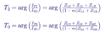
T2 applies to a negative-sequence-polarized reactance line and T0 to a zero-sequence-polarized line. For a loop-current-polarized element the corresponding angle depends on both the positive- and zero-sequence distribution factors and on the prefault load, which makes it hard to set securely. Neither T2 nor T0 depends on load, because the negative- and zero-sequence networks contain no load current.
These equations are evaluated for the system topology that produces the largest overreach risk, usually with the strongest remote source and the weakest local source in service, and with any parallel line in its worst state. The tilt is then entered as a downward correction (to prevent overreach) or an upward correction (to remove underreach), with the sign convention defined in the relay's instruction manual.
Worked Example 3: tilt for a non-homogeneous system
Use the same 230 kV line, with Zone 1 reactive reach at 80 percent, and consider two non-homogeneous systems with the same source magnitudes as Worked Example 2 but different angles:
- System A: local source at 86 degrees (Z1S = 12∠86°, Z0S = 30∠80°), remote source at 60 degrees (Z1R = 20∠60°, Z0R = 45∠60°).
- System B: local source at 60 degrees (Z1S = 12∠60°, Z0S = 30∠60°), remote source at 86 degrees (Z1R = 20∠86°, Z0R = 45∠80°).
Applying the T2 equation at m = 0.8 gives a tilt of +10.6 degrees for System A and −5.2 degrees for System B. The table shows the per-unit distance measured by a negative-sequence-polarized reactance line for an A-phase-to-ground fault exactly at the 80 percent reach point, with and without the calculated tilt.
| Fault resistance | System A, no tilt | System A, with T2 | System B, no tilt | System B, with T2 |
|---|---|---|---|---|
| 0 ohms | 0.800 | 0.800 | 0.800 | 0.800 |
| 10 ohms | 0.876 | 0.800 | 0.763 | 0.800 |
| 20 ohms | 0.951 | 0.800 | 0.726 | 0.800 |
| 30 ohms | 1.027 | 0.800 | 0.688 | 0.800 |
In System A, where the remote source angle is lower than the line angle, fault resistance makes the element underreach. At 30 ohms the fault at the reach point appears to be at 103 percent of the line, so the zone fails to operate for its own boundary fault. In System B the opposite happens: fault resistance makes the element overreach, and a 30-ohm fault at the 80 percent point appears at 69 percent. A fault well beyond the remote bus, with similar resistance, could therefore appear inside Zone 1. In both systems the calculated tilt removes the error completely for faults at the reach point.
Three practical observations follow:
- The tilt is exact only at the point and topology for which it is calculated. For faults at other locations or with other sources in service, a residual error remains. Most engineers calculate the tilt at the Zone 1 reach under the topology that produces the largest overreach and accept small underreach elsewhere.
- Overreach errors matter for Zone 1. Underreach errors matter for overreaching zones in pilot schemes. The tilt for Zone 2 is usually set equal to the Zone 1 tilt so the two reactance lines remain parallel, which preserves coordination for resistive faults.
- Instrument transformer angle errors add to the tilt requirement. Section 14 shows how a few degrees of measurement error limit the useful resistive reach.
Directional supervision
The directional boundary of a quadrilateral is rarely the only directional decision. Most relays also supervise ground zones with a negative-sequence or zero-sequence directional element. Negative-sequence directional elements are generally preferred when significant zero-sequence mutual coupling is present, because coupling corrupts both the zero-sequence voltage and current that a zero-sequence directional element uses. Zero-sequence directional elements can be advantageous where a strong local zero-sequence source, such as a large grounded transformer bank, makes the zero-sequence quantities large and stable, and where mutual coupling is absent.
Where inverter-based resources dominate the source behind the relay, negative-sequence quantities may be small or poorly controlled. In those cases zero-sequence directional elements, supported by the wye-grounded interconnection transformer, are often more dependable. Each case should be checked with a model that represents the plant's actual fault current behavior.
4. Comparing mho and quadrilateral elements
The two shapes side by side
Figure 1 shows the R-X plane for the 230 kV example. The black line is the protected line. The solid navy circle is a self-polarized Zone 1 mho set to 85 percent. The dashed circle is the same Zone 1 mho with memory polarization for forward faults, showing the expansion toward −ZS. The teal circle is Zone 2 at 125 percent. The magenta polygon is a Zone 1 quadrilateral with the same reactive reach and a 30-ohm resistive reach. The shaded region on the right is the load region for 1,600 A at 0.85 per unit voltage and a power factor angle of ±30 degrees. The gray trajectories show where A-phase-to-ground faults at 30, 70 and 100 percent of the line plot as fault resistance increases from 0 to 30 ohms.
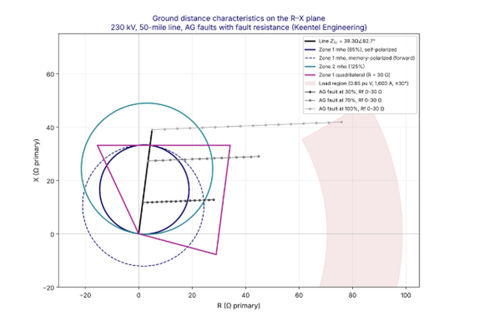
Figure 1. Ground mho and quadrilateral characteristics for the 230 kV, 50-mile example line, with fault resistance trajectories and the load region.
The figure makes several points visible at once. The self-polarized Zone 1 mho covers the 30 percent fault up to about 17 ohms of apparent resistance but the 70 percent fault only up to about 11 ohms. Memory polarization extends that coverage considerably. The quadrilateral covers both faults across the full 30-ohm range. All characteristics stay well clear of the load region. The 100 percent trajectory runs nearly horizontally above both Zone 1 characteristics, which is the correct behavior for a remote-bus fault.
Where each element is the better choice
The quadrilateral element has three structural advantages:
- Defined reactive reach. The reach along the line is a straight line, which makes coordination with adjacent lines easier to reason about.
- Independent resistive reach. The fault resistance coverage does not depend on the reactive reach. A short line can have a small reactive reach and a large resistive reach.
- Uniform coverage. The resistive coverage is the same at every point along the line, unlike the mho circle, which narrows toward its reach point.
The mho element has its own advantages:
- Load security. Its narrow shape near the reach point keeps it clear of load on long, heavily loaded lines without special settings.
- Fewer settings and fewer error sources. A mho element depends on reach and angle. A quadrilateral depends on reactive reach, resistive reach, tilt, polarizing method and directional angle.
- Resistive coverage comparable to quadrilaterals in pilot schemes. In a POTT or DCB scheme the overreaching zone is set long, often 150 to 200 percent of the line, so its circle is large and its resistive coverage at the line is substantial.
The comparison below summarizes Keentel's application guidance.
| Application | Preferred ground element | Reason |
|---|---|---|
| Long, heavily loaded line with pilot scheme | Mho | Load security, adequate coverage from the long pilot zone |
| Short line, strong sources, step distance only | Quadrilateral | Independent resistive reach recovers coverage the small mho circle lacks |
| High tower footing resistance, no shield wire, rocky or sandy soil | Quadrilateral, plus directional ground overcurrent | Fault resistance dominates |
| Single-pole tripping | Mho, or self-polarized quadrilateral | Sequence-polarized elements see open-pole unbalance |
| Parallel lines with strong mutual coupling | Either, with apparent-impedance-based reach and negative-sequence directional supervision | Coupling affects both shapes equally |
| Underground cable | Mho, if distance is used at all; line current differential preferred | Uncertain Z0 makes resistive reach unreliable |
| Series-compensated line | Relay designed for series compensation; settings tuned with hardware-in-the-loop testing | Voltage and current inversion dominate the decision |
| Line terminal with inverter-based resources | Mho with memory, quadrilateral with zero-sequence or loop polarizing; verify with IBR models | Negative-sequence quantities may be unreliable |
Ground distance versus ground overcurrent and differential
Neither distance shape matches the resistive sensitivity of a well-set directional ground overcurrent element, which can detect faults of several hundred ohms, or of a line current differential scheme, which compares currents directly and is unaffected by the voltage at the relay. Ground distance elements earn their place by providing a fixed, current-independent reach for fast tripping and for backup, while ground overcurrent and pilot schemes provide sensitivity. The best transmission line protection packages use all three.
How Keentel Engineering helps here: We select the ground element type for each line from a documented application matrix, calculate tilt and resistive reach from fault studies under credible topologies, and show clients exactly how much fault resistance each zone covers at each location along the line. That evidence supports protection philosophy decisions and settles debates with facts rather than habit.
5. Parallel lines and zero-sequence mutual coupling
The physics of mutual coupling
Current flowing in a transmission line creates a magnetic field around it, and that field induces a voltage in any nearby conductor that runs parallel to it. Between two three-phase circuits, the induced voltages from the three phase currents of one circuit largely cancel in the other circuit when the currents are balanced, because the three currents sum to zero and the three phase conductors are close together. That is why positive- and negative-sequence mutual coupling between transmission circuits is small, typically 3 to 7 percent of the self impedance, and is usually neglected in relay settings.
Zero-sequence current is different. Zero-sequence current is the same in all three phases and returns through the earth and the shield wires. Its magnetic field does not cancel, and the earth return path is shared by both circuits. As a result, the zero-sequence mutual impedance between two parallel circuits on the same structures is large, often 50 to 70 percent of the zero-sequence self impedance of either circuit. Even circuits on separate rights-of-way a few hundred feet apart can have zero-sequence mutual impedance of 20 to 40 percent of their self impedance.
The strength of zero-sequence coupling depends on:
- The length of the parallel section. Coupling is proportional to the length over which the circuits run together.
- The separation between the circuits. Coupling decreases slowly with distance, roughly with the logarithm of the separation, so circuits hundreds of feet apart can still be strongly coupled.
- Earth resistivity. Higher resistivity pushes the earth return current deeper and increases the mutual impedance.
- Shield wire configuration. Continuous, grounded shield wires carry part of the return current and slightly reduce the coupling.
- Transpositions and phase arrangement, which matter for positive-sequence coupling but have little effect on zero-sequence coupling.
What coupling does to the ground distance measurement
For an A-phase-to-ground fault at distance m on Line 1, with a parallel Line 2 carrying zero-sequence current I0M over the same section, the voltage at the Line 1 relay includes an extra term:
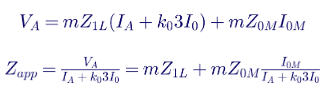
The second term is the mutual coupling error. Its sign depends on the direction of I0M relative to the relay's own residual current:
- Same direction (both lines feeding the fault from the same bus): the term adds, the apparent impedance increases, and the relay underreaches.
- Opposite direction (the parallel line current flows toward the relay bus): the term subtracts, the apparent impedance decreases, and the relay overreaches.
The magnitude of the error grows with the coupled length, the ratio Z0M/Z1L and the ratio of the parallel line residual current to the relay's compensated loop current. For faults near the remote bus of a double-circuit line, all three are at their maximum.
Why the fault study must model mutual impedance
Mutual coupling also changes the fault currents themselves. A short-circuit model that omits mutual impedances will show different 3I0 values on both circuits, sometimes by 10 to 30 percent, than a model that includes them. Directional ground overcurrent settings, ground distance reach calculations and ground current supervision thresholds based on a model without mutuals are therefore unreliable. Keentel's first check on any ground protection review is whether the short-circuit model includes every significant mutual impedance, including coupling between circuits at different voltages that share structures or corridors.
Eight coupling configurations every engineer should recognize
The effect of coupling depends on the network topology. The following eight configurations cover most situations found on US transmission systems. In each case "increase" means the relay sees the fault farther away (underreach risk) and "decrease" means it sees the fault closer (overreach risk).
| Case | Configuration | Effect on apparent impedance | Main risk |
|---|---|---|---|
| 1 | Two coupled lines between different buses, residual currents in the same direction | Increases | Overreaching zones underreach |
| 1 (reverse) | Two coupled lines with residual currents in opposite directions | Decreases | Zone 1 overreaches |
| 2 | Double-circuit line between the same two buses, fault on one circuit | Increases for remote faults, slightly decreases for close-in faults | Zone 2 and pilot underreach at the remote end |
| 3 | Double circuit plus a third parallel line connected to different buses | Circuits 1 and 2 increase each other's; the third line's opposing current decreases both | Combined errors that change with the third line's status |
| 4 | Partial coupling over part of the route, lines diverging to different buses | Depends on where the coupled section lies and which bus is common; can decrease at the common bus | Errors that a simple k0M correction cannot fix |
| 5 | Double circuit in which one circuit has an intermediate switching station | For a fault at the intermediate bus, one circuit's apparent impedance decreases and the other increases | Zone 1 overreach on one segment and underreach on another |
| 6 | Four or more parallel circuits | Interior circuits are coupled to more neighbors and see the largest errors | Settings that differ by circuit position |
| 7 | Current reversal after sequential clearing | Apparent impedance swings from increased to decreased when the near-end breaker opens | Zone 1 overreach and directional element misoperation during the reversal |
| 8 | Parallel line out of service and grounded at both ends | Decreases | Zone 1 overreaches the remote bus during maintenance |
Case 7 in detail: current reversal
Current reversal deserves special attention because it combines a reach error with a directional error. Consider two parallel lines between Bus S and Bus R, with a ground fault on Line 1 near Bus R. Before any breaker opens, the fault current flows from Bus S to Bus R on both lines, and the Line 2 relays at Bus S see a forward fault while those at Bus R see a reverse fault. When the Line 1 breaker at Bus R opens first, the entire fault current from Bus R now flows back along Line 2 to Bus S and then along Line 1 to the fault. Line 2 current reverses. The Line 2 relay at Bus R, which had been restraining for a reverse fault, now sees a forward fault, and the Line 2 relay at Bus S, which had seen a forward fault, now sees a reverse fault.
If the Bus R relay on Line 2 picks up its forward pilot element before the Bus S relay on Line 2 resets its forward element, a POTT scheme can trip the healthy Line 2. Pilot schemes protect against this with current reversal blocking logic, sometimes called transient blocking, which holds the reverse-looking element's blocking decision for a short time after it drops out. Ground distance settings must coordinate with that logic: the reverse zone at each terminal must reach beyond what the remote forward zone sees, and the blocking timers must cover the expected reversal interval.
Case 8 in detail: the grounded parallel line
When a parallel circuit is removed from service for maintenance, it is usually grounded at both ends, and often at the work location as well, for worker safety. A grounded circuit forms a closed loop through the earth. Zero-sequence current in the energized circuit induces a voltage in the grounded circuit, which drives a circulating current in the opposite direction. That induced current partly cancels the zero-sequence flux of the faulted circuit, lowering the effective zero-sequence impedance of the faulted circuit. The relay then sees the fault closer than it is.
The grounded case is easy to overlook because the parallel line is "out of service". Yet it is a normal, planned operating condition, and NERC misoperation reports have repeatedly included Zone 1 overreach events during parallel line maintenance outages.
Worked Example 4: a 345 kV double-circuit line
A 345 kV double-circuit line runs 40 miles between Bus S and Bus R on common towers. Each circuit has the following line constants:
- Z1 = 0.055 + j0.60 ohms per mile
- Z0 = 0.38 + j1.95 ohms per mile
- Z0M (between the two circuits) = 0.32 + j1.10 ohms per mile
The source impedances are Z1S = 10∠86°, Z0S = 20∠82° at Bus S and Z1R = 14∠85°, Z0R = 28∠80° at Bus R, in primary ohms.
Step 1. Line impedances and compensation factors.

The mutual impedance is 58 percent of the zero-sequence self impedance, typical for a double-circuit tower.
Step 2. Apparent impedance for faults on Circuit 1. A sequence-network model with the mutual impedance represented explicitly was solved for A-phase-to-ground faults on Circuit 1, with Circuit 2 in three states. The table lists the ratio of the reactance measured by the Bus S relay on Circuit 1 to the true reactance to the fault.
| Fault location on Circuit 1 | Circuit 2 in service | Circuit 2 out, grounded both ends | Circuit 2 open, not grounded | Circuit 2 in service, with k0M |
|---|---|---|---|---|
| 50% | 1.012 | 0.986 | 1.000 | 1.000 |
| 80% | 1.098 | 0.908 | 1.000 | 1.000 |
| 100% (remote bus) | 1.291 | 0.808 | 1.000 | 1.000 |
Figure 2 shows the same ratio continuously along the line.
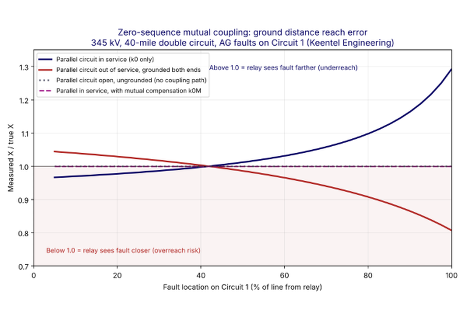
Figure 2. Reach error of the Circuit 1 ground distance element at Bus S for A-phase-to-ground faults along the line, for three states of the parallel circuit and with mutual compensation.
Step 3. Interpretation. With both circuits in service, a remote-bus ground fault appears 29 percent farther away than it is. A Zone 2 set to 125 percent of the line, with a reactive reach of 30.0 ohms, would not see a bolted remote-bus fault at all, because the fault appears at 31.0 ohms of reactance, and it would be even further from covering a remote-bus fault with resistance. With Circuit 2 out of service and grounded, the same fault appears at 81 percent of the line. A Zone 1 set to 85 percent of the line, 20.5 ohms, would trip instantaneously for a remote-bus fault (19.4 ohms apparent) and for faults on the lines beyond Bus R. With Circuit 2 open and ungrounded, the coupling has no closed path and the relay measures correctly.
Step 4. Settings. Following the apparent-impedance method:
| Zone | Basis | Calculation | Setting |
|---|---|---|---|
| Zone 1 | 85% of the lowest apparent X for a remote-bus fault (Circuit 2 grounded) | 0.85 × 0.808 × 24.10 | 16.6 ohms primary (69% of Z1L) |
| Zone 2 | At least 120% of the highest apparent X for a remote-bus fault (Circuit 2 in service) | 1.20 × 1.291 × 24.10 | 37.3 ohms primary (155% of Z1L), subject to coordination with Zone 1 of adjacent lines |
| Pilot overreach | Margin above Zone 2 | 2.0 × 24.10 | 48.2 ohms primary, check against reverse zone at Bus R |
The reduced Zone 1 is the price of security during maintenance. In practice many utilities with double-circuit lines use one of the alternatives described below rather than permanently shortening Zone 1.
Setting strategies for mutually coupled lines
There are five main ways to deal with mutual coupling, and they are often combined.
Strategy 1: apparent-impedance-based reach. Base underreaching zones on the lowest apparent impedance for a remote-bus ground fault across all credible states of the parallel line (in service, out of service and open, out of service and grounded). Base overreaching zones on the highest apparent impedance. Check faults on the parallel line near the remote bus as well, because some topologies produce a lower apparent impedance for those faults than for the remote-bus fault. This strategy is simple and robust but sacrifices Zone 1 coverage.
Strategy 2: mutual compensation (k0M). Wire the residual current of the parallel line into the relay and add k0M·3I0M to the loop current. This cancels the coupling term when the parallel line is in service and its current is measured. It does nothing for the grounded parallel line case if the parallel line's CTs are outside the grounded loop or if its breakers are open. Mutual compensation also creates an overreach risk for faults on the parallel line near the remote bus, where the parallel residual current is large and the relay's own current is small. Relays that offer k0M therefore usually include a supervision that disables mutual compensation when the parallel line residual current greatly exceeds the line's own residual current. Follow the relay maker's recommendations for applying k0M and its supervision, and apply it mainly to overreaching zones unless a fault study proves Zone 1 remains secure.
Strategy 3: a second compensation factor. Some relays allow a separate k0 for overreaching zones. Setting that k0 to include the effect of an in-service parallel line, for example k0' = (Z0L + Z0M − Z1L)/(3·Z1L) for a remote-bus fault fed equally by both circuits, extends the overreaching zones without changing Zone 1. Because the correct value depends on the current distribution, the second k0 must be validated with a fault study.
Strategy 4: adaptive setting groups. Bring the parallel line breaker status or disconnect status into the relay and switch to a setting group with a reduced Zone 1 when the parallel line is out of service. A grounding switch status input can specifically identify the grounded state. This recovers full Zone 1 coverage during normal operation but depends on reliable status inputs and must be tested as part of the protection system.
Strategy 5: pilot schemes. If a reliable pilot channel exists, a POTT or DCB scheme with properly set overreaching and reverse zones provides high-speed tripping for the whole line, and Zone 1 can be shortened without loss of speed. Line current differential protection is immune to mutual coupling and is often the simplest answer on heavily coupled double-circuit lines.
Directional element choice with mutual coupling
Zero-sequence mutual coupling affects both the zero-sequence voltage and the zero-sequence current at the relay. A zero-sequence voltage-polarized directional element can therefore make wrong decisions, especially on the healthy circuit of a double-circuit line during a fault on the other circuit, when the induced zero-sequence voltage can exceed the voltage from the relay's own current. Negative-sequence voltage polarization is preferred in the presence of significant mutual coupling, because negative-sequence coupling between circuits is small. Where negative-sequence quantities are too small, for example near large inverter-based resources, current polarization from a local grounded transformer neutral can be an alternative.
Coupling between circuits at different voltages
Coupling is not limited to circuits at the same voltage. A 69 kV line built under a 230 kV line, a 138 kV circuit on the lower arms of a 345 kV tower, or a 115 kV line sharing a corridor with a 500 kV line will be strongly coupled. The lower-voltage circuit usually has smaller fault currents and weaker sources, so the induced voltage from a fault on the higher-voltage circuit can dominate its relay's measurement. Directional ground overcurrent elements on the lower-voltage circuit can see a reverse-direction fault as forward, and ground distance elements can see a fault on the other circuit as internal. These interactions are frequently missed because the two circuits are planned and protected by different groups or even different companies.
How Keentel Engineering helps here: We build mutual coupling data from route geometry and corridor maps, add it to the short-circuit model, and run every parallel line state that operations and maintenance can create, including grounded outages. We then recommend the combination of apparent-impedance reach, k0M, setting groups and pilot logic that gives the client the best balance of speed and security, with every case documented for PRC-027 coordination records.
6. Weak sources and inverter-based resources
What makes a source weak for ground distance
A ground distance element needs enough current to measure reliably. Every relay supervises its ground zones with minimum current thresholds, usually a phase current detector and a residual current detector, to avoid operating on noise, CT errors and standing unbalance. If the available residual current at the relay for an internal fault is below that threshold, the ground distance zone cannot operate regardless of its reach.
A terminal can be weak in two different senses:
- Weak in positive and negative sequence. Few or no synchronous machines behind the relay, a long radial feed from a distant source, or a terminal that connects mainly to inverter-based resources. Phase current contributions are small.
- Weak in zero sequence. No grounded transformer neutral near the terminal, or a terminal whose only zero-sequence path is through a distant grounded bank. Residual current contributions are small even if phase currents are moderate.
A terminal can be strong in one sense and weak in the other. A solar plant interconnected through a wye-grounded/delta step-up transformer is a classic example: the transformer is a strong zero-sequence source, but the inverters behind it supply limited positive- and negative-sequence current.
An illustrative weak-source problem
Consider a 69 kV line, 14 miles long, that runs parallel to and is mutually coupled with a 138 kV line for most of its length. The local terminal, Station A, is fed through a single 138/69 kV transformer whose 69 kV winding is wye-grounded, but the system behind Station A is weak. A fault study gives the following quantities at the Station A relay for faults on the 69 kV line:
| Fault and system condition | Apparent ground impedance (primary ohms) | Phase current (A) | Residual current 3I0 (A) |
|---|---|---|---|
| Close-in fault, remote end open | Not applicable | 4,900 | 4,900 |
| Remote-end fault, strongest local source out of service | 38.6 | 410 | 62 |
| Remote-end fault, all equipment in service | 38.5 | 455 | 70 |
The relay uses 800:5 CTs (ratio 160), selected to carry the maximum line loading. Its ground distance residual current supervision has a minimum setting of 0.5 A secondary, which is 80 A primary. For a remote-end fault, the relay sees only 62 to 70 A of residual current. The ground distance Zone 2 cannot operate for remote-end faults even though the apparent impedance is well inside its reach. Lowering the CT ratio is not an option because of the load requirement.
Options for the weak terminal
Engineers have several tools for this problem, each with tradeoffs
.
Option 1: directional ground overcurrent in the pilot scheme. Most relays allow a forward directional ground overcurrent element (67G) to key a POTT scheme alongside the ground distance Zone 2. Its minimum pickup may be lower, for example 0.25 A secondary. In practice the pickup is set somewhat higher, say 0.35 A secondary (56 A primary), so that the forward element at one end coordinates with the more sensitive reverse element at the other end, which is needed for current reversal security. At 56 A the element would detect the 62 to 70 A remote-end fault, but with little margin, and the directional decision itself becomes marginal at such low quantities.
Option 2: sequential tripping. The remote terminal, which is strong, trips first. Once it opens, the weak terminal becomes the only source for the fault, the current distribution changes, and the weak terminal's ground elements see enough current to operate. Clearing is delayed by the remote breaker time plus the local relay time, which is often acceptable for low-current faults whose damage potential is small. The study must confirm that the weak terminal can in fact detect the fault after the remote end opens.
Option 3: weak-infeed echo and trip logic. In a POTT scheme, a weak terminal that receives a permissive signal, does not see a reverse fault, and does not have enough current to key its own forward elements can echo the permissive signal back to the strong terminal, allowing it to trip at high speed. With weak-infeed trip logic, the weak terminal can also trip itself if it detects a low phase voltage or a zero-sequence voltage above a threshold. The zero-sequence voltage threshold may be near the bottom of the relay's setting range at weak terminals, so the low phase voltage condition is often the more useful one. Echo logic complicates current reversal coordination on parallel lines and must be tested carefully.
Option 4: a quadrilateral or extended zone. If the relay allows independent ground mho and ground quadrilateral zones, a timed Zone 2 quadrilateral can provide coverage for high-resistance ground faults ahead of the slower time-overcurrent backup, which in many systems coordinates at around 1 second. Its reactive reach is set like the mho Zone 2, and its time delay matches the Zone 2 timer used for coordination. This option does not solve the residual current supervision limit, but it adds resistive coverage once current is sufficient.
The most robust answer is often a combination: weak-infeed echo for high-speed tripping, a 67G element for sensitivity, and a timed ground zone for backup. On the coupled 69 kV and 138 kV pair, the current reversal coordination of both pilot schemes must be verified together, because sequential opening of the faulted line's terminals suddenly reverses current on the unfaulted line.
Inverter-based resources
Inverter-based resources present a newer and more complex version of the weak-source problem. Their fault current is limited by the inverter's semiconductor ratings, typically 1.0 to 1.5 times rated current, and its phase angle and sequence composition are set by the inverter's control system rather than by machine physics.
The main consequences for ground distance protection at an IBR interconnection are:
- Limited positive-sequence current. The IBR terminal of a generator tie line may see little phase current for faults on the line, which challenges fault detectors and phase selection.
- Controlled negative-sequence current. Older inverters often suppressed negative-sequence current entirely. IEEE 2800-2022 now requires IBRs interconnected to transmission systems to inject negative-sequence current during unbalanced faults with a phase relationship to negative-sequence voltage that resembles a synchronous machine. Plants built before that standard, or plants whose equipment is not fully compliant, may still inject little or poorly controlled negative-sequence current.
- Strong zero-sequence path. The wye-grounded high-voltage winding of the main power transformer supplies residual current like any grounded transformer. Ground distance and zero-sequence directional elements usually perform better than negative-sequence elements at the IBR terminal.
- Unusual fault-type selection. Fault-type selection logic that relies on the angle between negative- and zero-sequence currents may choose the wrong loop when the negative-sequence current is small or phase-shifted. Voltage-based fault-type selection helps.
- Source impedance is not a constant. The apparent source impedance seen from the line changes during the fault as the inverter control responds. The SIR at the IBR terminal is therefore not well defined and can be very high.
- CVT transient sensitivity. Because the terminal can behave like a very weak source, Zone 1 elements at the IBR end may need CVT transient security logic even on lines that would not be considered short.
Keentel treats IBR interconnections as an EMT problem as well as a phasor problem. Short-circuit programs with IBR models based on voltage-controlled current sources give a good first estimate, but the behavior of the relay's fault-type selection and directional logic in the first two cycles is best confirmed with EMT simulation of the actual inverter models and, for critical applications, with hardware-in-the-loop testing of the relay.
How Keentel Engineering helps here: We identify weak terminals in fault studies under N-1 conditions, quantify the residual current margin at every relay, and design the combination of 67G, weak-infeed logic, sequential tripping and timed ground zones that gives dependable clearing. For IBR interconnections we use manufacturer-specific inverter models in both short-circuit and EMT studies, consistent with the plant's IEEE 2800 performance, to set and verify ground distance and directional elements at the point of interconnection.
7. Instrument transformer transients: CVTs, CT saturation and inrush
Distance elements are only as good as the voltages and currents they receive. Three instrument transformer phenomena matter most for ground distance elements: transients from coupling capacitor voltage transformers, saturation of current transformers, and false residual current during transformer energization.
How a CVT works
A coupling capacitor voltage transformer uses a capacitive voltage divider, made of a high-voltage capacitor stack C1 and a tap capacitor C2, to bring the line voltage down to an intermediate level, typically 5 to 20 kV. A tuning reactor in series with the divider output cancels the divider's capacitive reactance at 60 Hz, and a step-down transformer reduces the voltage to the 115 V or 67 V secondary used by relays. A ferroresonance suppression circuit across the secondary prevents sustained subharmonic oscillation between the capacitors and the nonlinear transformer core.
CVTs are economical and compact at 115 kV and above. They can double as coupling capacitors for power line carrier channels, and their capacitance can improve the transient recovery voltage duty of nearby breakers. Those advantages explain why they dominate high-voltage protection applications in the US. Their weakness is that the capacitors and inductors store energy, and that energy cannot disappear instantly when the primary voltage collapses during a fault.
The CVT transient
When a fault causes the primary voltage to collapse, the energy stored in the capacitor stack, the tuning reactor, the step-down transformer and the ferroresonance circuit discharges through the secondary burden. For one to two cycles the secondary voltage does not follow the primary. It contains a decaying low-frequency or subsidence transient that can be a significant fraction of the prefault voltage.
Six factors determine the size and duration of the transient:
| Factor | Effect on transient |
|---|---|
| Point on wave of fault inception | Worst near a voltage zero crossing, when the stack capacitance holds maximum stored energy relative to the instantaneous voltage; mildest near a voltage peak |
| Total capacitance (C1 + C2) | Higher capacitance lowers the transient amplitude but can lengthen its duration; high-capacitance CVTs generally perform better |
| Ferroresonance suppression circuit type | Active (tuned L-C) circuits add a band-pass response and delay; passive (resistive) circuits produce less distortion |
| Secondary burden magnitude | Larger burden stores more energy and increases the transient |
| Secondary burden power factor | Inductive burdens make the transient more oscillatory at subnominal frequency |
| Step-down transformer excitation | Magnetizing current and core behavior shape the low-frequency component |
Why the CVT transient makes Zone 1 overreach
A distance relay filters the secondary voltage to extract the 60 Hz phasor. During the CVT transient, the filtered voltage magnitude dips below the true primary value for roughly 1 to 1.5 cycles, and its angle shifts. The relay divides that low voltage by a correctly measured current and calculates an impedance smaller than the true impedance. For a fault just beyond the remote bus, the computed impedance can briefly fall inside Zone 1. Because Zone 1 trips without intentional delay, that brief excursion is enough to cause an overreach trip.
The effect is greatest when the relay voltage for a remote fault is already small, which is the high-SIR condition. On a long line with a strong source the fault voltage at the relay is a large fraction of nominal, and the transient is a small fraction of it. On a short line or a weak source, the fault voltage is small and the transient can dominate it. Zone 2 and Zone 3 elements are not affected because their time delays are longer than the transient.
Mitigating CVT transients
| Strategy | How it works | Tradeoffs |
|---|---|---|
| Reduce Zone 1 reach | Leave enough margin that the transient cannot pull the computed impedance inside the zone | Less high-speed coverage; at very high SIR, the secure reach may be shorter than the relay's minimum setting |
| Add a short Zone 1 delay | Delay of about 1 to 2 cycles outlasts the transient | Slower clearing for all Zone 1 faults |
| Disable Zone 1 | For very high SIR lines where no secure reach exists | Depends entirely on pilot or Zone 2 clearing |
| Adaptive CVT transient detection in the relay | The relay detects high-SIR conditions from its own measurements and applies extra filtering or a short delay only when needed, while still tripping fast for close-in faults | Must be enabled and set per the relay maker's guidance; performance varies between designs |
| Choose better CVTs | Specify high-capacitance CVTs with passive ferroresonance suppression and low, resistive burdens | Equipment cost; applies to new installations and replacements |
| Use pilot protection | Zone 1 becomes less important when POTT, DCB or line current differential provides high-speed tripping | Requires a reliable channel |
Published industry experience indicates that with active ferroresonance suppression, Zone 1 reach reduction is generally not required for SIRs up to about 4, while at very high SIRs, in the range of 20 to 30, a secure Zone 1 may not exist without transient-blocking logic. Passive suppression extends the usable range. These thresholds vary with relay filtering and should always be checked against the relay maker's published performance for the specific CVT class.
CT saturation and the distance measurement
A current transformer saturates when the flux required to reproduce the primary current exceeds what its core can support. The DC offset in fault current is the main cause: an asymmetrical fault on a high X/R system requires the CT core to carry a flux many times greater than the symmetrical fault would require. When the core saturates, the secondary current collapses for part of each cycle, and the relay's filtered phasor shows both a reduced magnitude and a phase shift, usually a phase advance.
For a distance element, a smaller measured current means a larger computed impedance. Saturation therefore makes distance elements underreach. Security is not usually threatened: a saturated CT does not make an external fault look internal. Dependability is threatened: a fault that should be inside Zone 2 may temporarily appear outside it, causing the zone to drop out and its timer to reset, and a pilot zone may assert later than expected. When the CT recovers, the measurement returns to its true value, but the clearing time has already been extended.
The phase shift caused by saturation can also disturb directional decisions and the angle comparisons used in fault-type selection, which is why severe saturation on the residual circuit deserves attention even when the reach effect seems acceptable.
CT sizing equations
The IEEE C37.110 criterion for avoiding saturation entirely with a fully offset fault is:
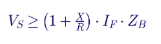
where VS is the CT saturation voltage (approximately its C-class rating at 20 times rated current), IF is the secondary fault current, X/R is the reactance-to-resistance ratio of the fault path, and ZB is the total secondary burden including the CT winding resistance, leads and relay. For high-X/R transmission faults this criterion often cannot be met with practical CTs.
Distance elements tolerate some saturation, because they only need correct measurement for the time it takes to operate. A widely used industry criterion for distance elements in pilot schemes states that a Zone 2 element set to 125 percent of the line will operate correctly for a fault at 100 percent of the line if the burden satisfies:
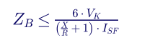
where VK is the CT voltage rating and ISF is the maximum secondary fault current. This relaxed criterion is roughly six times more permissive than the saturation-free criterion. It should be checked against the relay maker's own guidance for the specific relay.
The time to saturate can be estimated from the IEEE C37.110 approach. Defining the saturation factor KS as the ratio of saturation voltage to the symmetrical burden voltage:

The equation applies when KS is less than 1 + X/R. Remanent flux in the core shortens the time to saturate and can be significant after a previous fault or after DC testing.
Worked Example 5: CT performance for a 230 kV line relay
A 230 kV line terminal has a maximum close-in ground fault current of 40 kA with an X/R ratio of 20. The relay uses 2000:5 multi-ratio C800 CTs at full ratio. The total secondary burden is 1.5 ohms, including CT winding resistance, leads and relay.
Step 1. Secondary fault current. 40,000 / 400 = 100 A secondary.
Step 2. Saturation-free requirement.

A C800 CT cannot avoid saturation for a fully offset close-in fault.
Step 3. Time to saturate.

The CT saturates in under one cycle for the worst-case offset. For a close-in fault this is acceptable, because Zone 1 and the pilot elements will usually operate within the first cycle, and the fault is deep inside the zone.
Step 4. Distance element criterion.

The actual burden of 1.5 ohms meets the distance criterion with margin. The table shows how the time to saturate improves if the burden is reduced.
| Total burden | KS | Estimated time to saturate |
|---|---|---|
| 1.5 ohms | 5.3 | 0.8 cycle |
| 1.0 ohm | 8.0 | 1.4 cycles |
| 0.5 ohm | 16.0 | 4.4 cycles |
Reducing burden, for example by using larger lead wire, eliminating auxiliary CTs and placing relays closer to the CT, is usually the cheapest way to improve CT performance.
Mitigating CT saturation effects
- Size CTs for the overreaching zone. The overreaching pilot zone and the Zone 2 element must assert dependably for remote-end faults, where the fault current and its DC offset are smaller than for close-in faults. That is the governing criterion for distance relays.
- Do not simply extend reach. If saturation can reduce the current magnitude by more than about 30 percent, adding extra margin to Zone 2 reach to compensate is unwise, because it can create overreach problems for remote faults when the CT does not saturate.
- Use dropout extension timers. A short dropout timer on Zone 2 holds the element picked up through brief excursions caused by saturation, so the zone timer is not reset. A second timer can then trip if the zone has been picked up, with the extension, for the full Zone 2 time.
- Use the CT at full ratio. Using a tap of a multi-ratio CT reduces its effective voltage rating in proportion to the turns used.
- Watch the residual circuit. Unequal saturation of the three phase CTs produces false residual current, which affects ground distance compensation, directional elements and ground overcurrent elements.
Transformer inrush
When a line that feeds a transformer is energized, the transformer can draw magnetizing inrush current of several times its rating for many cycles. Inrush is rich in second harmonic and contains a large DC component. For phase distance elements, inrush current with depressed voltage can occasionally produce an impedance that plots inside a long zone. Ground distance elements are rarely affected by genuine inrush, because inrush current contains little true zero-sequence current. The concern is false residual current produced by unequal CT saturation during inrush, especially when the DC component persists for many cycles. If the line terminates directly at a transformer, CT sizing should be checked using the inrush current in place of the fault current, although the maximum fault current is usually larger and remains the governing case.
How Keentel Engineering helps here: We review CVT specifications and burdens, calculate SIRs under N-1 conditions, and recommend Zone 1 reach, delays or relay transient logic that keep Zone 1 secure. We perform CT saturation studies to IEEE C37.110 methods, including time-to-saturate and remanence analysis, and we specify CT ratios, accuracy classes and burdens for new substations and upgrades.
8. Faulted phase selection
Why phase selection matters
A distance relay evaluates all six fault loops continuously, but for any given fault only some loops measure the true fault impedance. The others see distorted apparent impedances that can still plot inside a zone. Faulted phase selection is the logic that decides which loops are valid for the fault in progress, so the relay trips correctly, reports the right fault type, selects the right phase for single-pole tripping and locates the fault accurately.
Phase selection is not a setting the user chooses. It is designed into the relay. But the user's settings, especially resistive reaches and ground current thresholds, affect how well it works, and the application engineer must understand where it can fail.
Which loops measure correctly
| Fault type | Example | Loops that measure correctly |
|---|---|---|
| Phase-to-phase without ground | B-C | BC only |
| Three-phase without ground | A-B-C | AB, BC or CA |
| Single-phase-to-ground | B-G | BG only |
| Phase-to-phase-to-ground | B-C-G | BG, CG or BC, depending on fault resistance |
| Three-phase-to-ground | A-B-C-G | Any of the six loops |
For a single-line-to-ground fault, only one loop is valid. The two phase loops that include the faulted phase also see a reduced voltage and an increased current, and for close-in faults their apparent impedances can fall inside a zone. Without good phase selection, a ground fault near a strong source can trip three poles when only one should open, or be reported as a phase-to-phase fault.
Phase selection methods
| Method | Principle | Weakness |
|---|---|---|
| Current magnitude | Faulted phases carry more current than healthy ones | Fails with weak infeed; misled when residual current is distorted by CT saturation |
| Voltage magnitude | Faulted phase voltages collapse | Fails with strong sources and low SIR, where the voltage drop is small |
| Delta current | Change of current from prefault values identifies faulted phases | Weak infeed; sensitive to load changes |
| Delta voltage | Change of voltage from prefault values | Switch-onto-fault cases with no prefault memory; non-fault transients |
| Impedance comparison | The loop with the lowest impedance relative to the others is the faulted loop | "Ghost" impedances in non-faulted loops close to the zone boundary |
| Symmetrical components | Angle between negative- and zero-sequence currents identifies the faulted phase or phase pair | Fails when the sequence currents do not come from the fault, such as during open-pole intervals or with inverters that inject little negative-sequence current |
| Jump detection | Combination of sudden current and voltage changes | Transients not related to the fault |
Modern relays usually combine several methods and choose the faulted loop only when they agree, which greatly improves reliability. The symmetrical component method, based on the angle between I2 and I0, is common. For an A-phase-to-ground fault in a homogeneous system, I2 and I0 for the A phase are nearly in phase. For a B-phase or C-phase fault, I2 is rotated by 120 degrees from I0. Fault resistance and non-homogeneity shift those angles, and a design must allow a sector of perhaps ±30 to 60 degrees around each nominal angle.
Practical setting considerations
- Phase loop resistive reach near strong sources. If the phase quadrilateral resistive reach is very large, a close-in ground fault can make a phase loop that includes the faulted phase appear inside Zone 1. Limiting the phase loop resistive reach, for example to a value comfortably below the apparent resistance of a close-in ground fault on the healthy loop, prevents a three-pole trip for a single-line-to-ground fault. Faults involving two phases rarely need the large resistive coverage that ground loops do.
- IBR terminals. Where inverters supply little negative-sequence current, phase selection that depends on I2 and I0 angles can fail. Voltage-based phase selection improves security in those cases. Check the relay's behavior with an IBR model.
- Open-pole conditions. During single-pole dead time, the sequence currents come from the open-phase unbalance rather than from a fault. Phase selection must be blocked or modified during the open-pole interval (Section 11).
- Event reports. Phase selection decisions appear in relay event reports. Reviewing them after every ground fault is a simple way to detect a phase selection problem before it causes a misoperation.
How Keentel Engineering helps here: We review relay event records to confirm phase selection behavior, adjust phase and ground resistive reaches to protect phase selection near strong sources, and test phase selection logic with playback of real and simulated fault records, including IBR fault signatures.
9. High SIR and short lines
Defining SIR
The source-to-line impedance ratio is the ratio of the source impedance behind a relay to the impedance of the protected line:

IEEE C37.113 uses SIR to classify line length for protection purposes: a line with an SIR below 0.5 is considered long, an SIR between 0.5 and 4 is medium, and an SIR above 4 is short. The classification depends on the source as well as the line. A 30-mile 138 kV line fed from a weak station can be electrically short, while a 3-mile 345 kV line next to a large generating plant can be electrically medium.
SIR is best calculated from a fault study rather than estimated from separate source and line impedances. For a homogeneous system, the relay voltage for a bolted fault at the remote bus is:

so the SIR can be obtained from the relay voltage reported by the short-circuit program. The phase-to-ground voltage for a ground fault at the remote bus gives the ground SIR used for ground distance elements. The phase-to-phase voltage for a phase-to-phase or three-phase fault gives the phase SIR. The two values differ when the zero-sequence source and line impedances have different ratios than the positive-sequence ones.
SIR is not fixed. When a generator or a transformer behind the relay is out of service, the source weakens and the SIR rises. A line that is medium under normal conditions can become short under N-1 conditions. The table shows an illustrative set of SIR calculations for lines on one US system.
| Voltage | Length | SIR (all in service) | SIR (N-1) |
|---|---|---|---|
| 69 kV | 6.0 miles | 0.8 | 1.4 |
| 69 kV | 1.5 miles | 11.8 | 46.0 |
| 115 kV | 9.5 miles | 1.3 | 2.1 |
| 138 kV | 8.0 miles | 2.6 | 17.5 |
| 230 kV | 22.0 miles | 0.9 | 3.2 |
| 345 kV | 18.0 miles | 2.8 | 8.4 |
Two observations stand out. Physical length is a poor predictor of SIR: a 138 kV line of 8 miles has a higher N-1 SIR than a 69 kV line of 6 miles. And the N-1 condition can raise the SIR by a factor of five or more.
Why high SIR makes distance measurement harder
At high SIR, the relay voltage for a fault near the reach point is small. Any error in the voltage measurement, whether from the CVT transient, the VT ratio and angle accuracy, the relay's own measurement error, or the arc voltage, becomes a large fraction of the measured voltage. The resulting impedance error grows roughly in proportion to 1 + SIR.
Worked Example 6: measurement error versus SIR
Suppose the combined steady-state voltage measurement error at the relay is 1 percent of nominal voltage. The table shows the resulting impedance error for a fault at the remote bus at different SIRs. The relay voltage is calculated from the homogeneous expression above.
| SIR | Relay voltage for remote-bus fault | Impedance error from 1% voltage error | Impedance error from 0.5% voltage error |
|---|---|---|---|
| 0.5 | 0.667 pu | 1.5% | 0.8% |
| 1 | 0.500 pu | 2.0% | 1.0% |
| 2 | 0.333 pu | 3.0% | 1.5% |
| 4 | 0.200 pu | 5.0% | 2.5% |
| 10 | 0.091 pu | 11.0% | 5.5% |
| 20 | 0.048 pu | 21.0% | 10.5% |
| 30 | 0.032 pu | 31.0% | 15.5% |
At SIR 30, a 1 percent voltage error becomes a 31 percent impedance error. A Zone 1 set to 85 percent of the line has only 15 percent of margin and cannot accommodate that error. This is why underreaching zones must be pulled back, delayed or disabled on high-SIR lines, independently of the CVT transient issue.
Steady-state errors from wound VTs
CVT transients get most of the attention, but wound (magnetic) VTs also contribute steady-state ratio and phase angle errors, defined by their accuracy class. For VTs the dominant concern is steady-state, so a line that is physically short, with a small absolute impedance, can be more problematic than one that is merely electrically short. Small absolute errors in line constants, CT and VT ratios and relay measurement add up to a large fraction of a small reach.
When VTs are wye-connected and measure phase-to-ground voltages, their angle errors can also combine unfavorably for phase-to-phase loops. The reach of phase distance elements may need to be reduced more than that of ground distance elements on very short lines.
Arc voltage at high SIR
For ground faults, the arc and fault resistance add a voltage that is essentially in phase with the fault current. On a long line with low SIR, this voltage is small compared with the line voltage drop. On a short line with high SIR, the line voltage drop is small, and the arc voltage can become a large fraction of the relay voltage. Depending on the phase relationship between the relay current and the total fault current, the arc can make the relay overreach or underreach. Zone 1 may need to be pulled back further on short lines to account for this effect, even with good instrument transformers.
Practical guidance for short lines
- Use pilot protection. Line current differential, POTT, DCB and phase comparison schemes all work well on short lines. When a reliable pilot channel is available, an underreaching Zone 1 may not be needed at all.
- If Zone 1 is used, set it with a margin calculated from the SIR. For example, with an expected total measurement error of 1 percent of nominal voltage and SIR 10, the error is about 11 percent, so Zone 1 might be set to about 75 percent of the line rather than 85 percent.
- Use the relay's CVT transient logic on high-SIR lines with CVTs, and verify its operating time for close-in faults.
- Quadrilateral resistive reach must shrink too. Pulling back Zone 1 reactive reach reduces the allowable resistive reach (Section 14), so short lines rarely support the large resistive coverage that would otherwise justify a quadrilateral.
- Consult the relay maker's published accuracy data for the specific relay model and filtering when SIR exceeds about 10.
How Keentel Engineering helps here: We calculate phase and ground SIRs for every line terminal under normal and N-1 conditions, flag the terminals where measurement error and CVT transients threaten Zone 1 security, and recommend reach, delay or pilot scheme solutions. For short lines we often recommend line current differential with distance backup and provide the full setting package.
10. Underground cables
Why cables are different
Underground transmission cables are common in US urban areas, at river crossings, at substations with overhead line entrance constraints, and increasingly at data center campuses where aesthetic, security or right-of-way limits rule out overhead lines. Cables fail differently from overhead lines. Most cable faults involve ground. They are almost never temporary, so reclosing is usually blocked. Repair takes far longer than for an overhead line, often three to five times longer, because the fault must be located and the cable excavated, spliced and tested. For pipe-type cables, a fault that is not cleared quickly can burn through the steel pipe and release the insulating fluid. Fast, dependable ground fault protection is therefore essential.
Line current differential protection is the usual choice for high-voltage cables. Directional comparison schemes with negative-sequence directional elements are also used and perform well, because the negative-sequence impedances of cables are stable and predictable. Zero-sequence directional elements are generally not recommended for cables, because the zero-sequence impedance is uncertain. Ground distance elements are often applied as backup, and sometimes as the main pilot elements, but they face unique challenges.
Electrical characteristics of cables
| Characteristic | Overhead line | Underground cable |
|---|---|---|
| Positive-sequence series reactance per mile | About 0.6 to 0.8 ohms | Typically 30 to 50 percent lower |
| Shunt capacitance per mile | Baseline | Often 30 to 40 times higher |
| Zero-sequence impedance | Roughly proportional to length; determined mainly by earth return | Depends on sheath bonding, sheath resistance, earth resistivity and nearby metallic paths; may be nonlinear with distance |
| Zero-sequence impedance angle | Typically 70 to 80 degrees | Can be as low as 10 to 40 degrees for sheath return paths |
| k0 | Small angle, magnitude about 0.6 to 0.8 | Magnitude and angle vary widely; angle can be large and negative |
Ground return paths and nonlinearity
A single-conductor cable has a metallic sheath or concentric neutral wires that are grounded at one or more points. During a core-to-sheath fault, the return current can flow through the faulted cable's sheath, through the sheaths of the other two phases, through the earth, through a separate ground continuity conductor, and through any nearby water pipes, gas pipes or adjacent cable circuits. How it divides depends on the bonding method and on where the fault is.
- Solidly bonded sheaths (grounded at both ends) give a continuous return path. The compensated ground loop impedance varies smoothly but nonlinearly with fault location.
- Cross-bonded sheaths (transposed at each minor section and grounded at the major section ends) create discontinuities. Moving a fault from the end of one minor section to the start of the next changes the return path abruptly, and the compensated loop impedance jumps. The maximum compensated resistance may not occur for a fault at the remote end.
- Single-point bonded sheaths force the return current through the earth or a ground continuity conductor and produce yet another characteristic.
- Pipe-type cables have a steel pipe whose permeability changes with current. Their zero-sequence impedance varies with the magnitude of the ground fault current itself, which makes the problem nonlinear in a second way.
Because the relay uses a single k0 value, no setting compensates correctly for every fault location and return path. Symmetrical component fault studies also struggle with cables, because the bonding arrangements make the cable impedances unbalanced. Accurate analysis uses a phase-domain model that retains the sheaths, their transpositions and their grounding, and solves faults along the cable, ideally in an electromagnetic transients program or a phase-domain short-circuit tool. Field measurement of cable zero-sequence impedance during commissioning is good practice.
Worked Example 7: how much the k0 choice matters for a cable
A 230 kV underground cable is 3 miles long. Its positive-sequence impedance is 0.025 + j0.28 ohms per mile. Its zero-sequence impedance depends on the return path:
| Return path | Z0 per mile | Total Z0 | Corresponding k0 |
|---|---|---|---|
| Sheath only | 0.30 + j0.10 | 0.95∠18.4° | 0.39∠−118.1° |
| Sheath and earth in parallel | 0.26 + j0.22 | 1.02∠40.2° | 0.29∠−99.2° |
| Earth only | 0.25 + j1.60 | 4.86∠81.1° | 1.59∠−4.6° |
The positive-sequence impedance is 0.84∠84.9° ohms, a very small number that already challenges distance measurement. To isolate the effect of k0, consider a bolted fault at the remote end of the cable fed radially from the relay end, so that the relay currents are I1 = I2 = I0. The relay then measures:
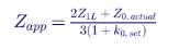
The table shows the measured reactance divided by the true positive-sequence reactance for each combination of set k0 and actual return path. Values below 1.0 mean overreach; values above 1.0 mean underreach.
| k0 set for | Actual: sheath only | Actual: sheath and earth | Actual: earth only |
|---|---|---|---|
| Sheath only | 1.00 | 1.13 | 2.83 |
| Sheath and earth | 0.88 | 1.00 | 2.58 |
| Earth only | 0.31 | 0.37 | 1.00 |
The consequences are dramatic. If k0 is set for earth return but the current actually returns through the sheath, the relay measures the fault at 31 percent of its true distance, a gross overreach. If k0 is set for sheath return but the current returns through the earth, the relay measures the fault at nearly three times its true distance.
These results lead to the setting principles for cables:
- For underreaching zones, choose the k0 that does not overreach for any credible return path. In this example that is the sheath-only k0, which never measures below 1.00. The underreaching zone may then fail to operate for faults with earth return, which must be accepted or covered by another element.
- For overreaching zones in pilot schemes, choose the k0 that does not underreach for any internal fault. In this example that is the earth-only k0, which always measures at or below 1.00. Because it can overreach, it is suitable only where the pilot scheme provides security; it is not suitable for time-delayed step-distance backup that must coordinate with adjacent zones.
- Use a complex k0 with a wide angle range, or a fictitious scalar k0 chosen to give correct reach at the end of the cable, if the relay offers it.
- Prefer negative-sequence current polarization and negative-sequence directional elements, because the negative-sequence network is more homogeneous and predictable.
- Mho elements generally perform better than quadrilateral elements on cables, because they are less sensitive to errors in the resistive component of the compensated loop impedance.
Mixed overhead and cable circuits
Hybrid circuits that combine overhead and underground sections are increasingly common, for example where an overhead line transitions to cable near a substation or under a highway. The zero-sequence impedance per unit length changes abruptly at each transition, and the cable section's nonlinear behavior affects measurements for faults in the overhead section beyond it.
Setting a single k0 for the whole circuit is a compromise. Each section must be modeled, faults applied throughout each section, and the zones checked against the worst-case measurements.
For parallel cable circuits between the same two substations, select the Zone 1 k0 by applying a remote-terminal ground fault with the parallel cable out of service and checking the measurement for both the sheath-only and the sheath-and-earth return paths. Select the overreaching zone k0 by applying the same fault with both cables in service and checking all three return paths.
How Keentel Engineering helps here: We model cable systems in the phase domain with their actual bonding and grounding, compute compensated loop impedances along the cable and through hybrid transitions, and recommend whether ground distance is appropriate at all. Where it is, we choose the k0, polarizing and zone settings from those studies; where it is not, we design line current differential or negative-sequence directional comparison schemes for the cable.
11. Single-pole tripping and open-pole conditions
Why single-pole tripping is used
Most faults on overhead transmission lines are temporary single-line-to-ground faults caused by lightning, wind or contamination. If the breakers have independent pole mechanisms, the relay can open only the faulted phase, wait for the arc to deionize, and reclose that phase while the other two phases continue to carry power. Single-pole tripping and reclosing offers three main advantages over three-pole tripping:
- Power continues to flow on the two healthy phases during the dead time, so the transfer capacity of the corridor is largely maintained.
- The risk of loss of synchronism and power swings is reduced, which improves transient stability.
- The two ends of the line remain synchronized, so the reclose can be performed without a synchronism check.
In the US, single-pole tripping is used mainly on long EHV lines at 345 kV, 500 kV and 765 kV, on lines that are critical for stability, and on some long 230 kV lines. Dead times are typically 0.5 to 1.5 seconds, long enough for the secondary arc, which is sustained by capacitive coupling from the energized phases, to extinguish. Long lines may need shunt reactors with neutral reactors to suppress the secondary arc.
What the open pole does to the network
When one phase of a line is open, the line becomes an unbalanced element. Load current that flowed in the open phase must find another path. On parallel lines, it transfers to the corresponding phase of the parallel circuit, so the parallel line carries significant zero- and negative-sequence current even though it has no fault. On the faulted line itself, the two healthy phases continue to carry load, and residual current flows in the line.
In one recorded event on a pair of parallel transmission lines, the peak phase current on the unfaulted parallel line rose from about 750 A before the fault to about 1,350 A during the single-pole dead time, and both lines carried substantial neutral current throughout the open-phase interval, which lasted almost 1.5 seconds.
Risks for ground distance elements on the parallel line
On the unfaulted parallel line, sensitive and long-reaching ground elements, such as an extended Zone 3 or a sensitive ground overcurrent element, can see the open-phase unbalance under heavy load. If their time delay is shorter than the dead time of the faulted line's reclosing cycle, they can trip the healthy line. The usual remedy is to set the time delay of such elements longer than the single-pole dead time plus margin. For a 1.0-second dead time, a delay of about 1.3 to 1.5 seconds is common. The required delay depends on the actual dead time used, which differs between systems and between lines.
Challenges on the faulted line
On the faulted line, the distance relay must handle three challenges during a single-pole trip.
Correct phase selection. A wrong phase selection would open the wrong pole or trip three poles unnecessarily. For a close-in A-phase-to-ground fault near a strong source, the AB and CA phase loops can see apparent impedances near or inside Zone 1. If phase selection is not robust, the phase loop elements may operate and force a three-pole trip. Reducing the phase loop resistive reach of Zone 1, for example from a generous value to around 10 ohms in one documented case, can keep those loops out of Zone 1 for close-in ground faults while still covering genuine phase faults.
Stability during the dead time. With one pole open, the healthy phases carry load and the network carries zero- and negative-sequence currents caused by the open phase. The apparent impedances of the healthy ground loops can move into the zones, particularly on long, heavily loaded lines. The relay must detect the open-pole condition and block or modify the ground loops that would otherwise respond to the unbalance. Negative- and zero-sequence directional elements and sequence-polarized quadrilateral elements are especially vulnerable, because the sequence quantities during the dead time come from the open phase rather than from a fault.
Detecting evolving faults. A second fault on a healthy phase during the dead time must be detected and cleared quickly, normally by tripping all three poles. The relay must distinguish a genuine new fault, whose impedance appears in a forward zone on the newly faulted loop, from the open-pole unbalance, which may make a healthy loop plot in a reverse zone or near a zone boundary. Modern relays switch to an open-pole measurement mode that uses only the valid loops and compensates for the open-phase unbalance.
Detecting the open-pole state
Relays detect a single-pole-open condition from several inputs, often in combination:
- The relay's own single-pole trip command.
- Breaker auxiliary contacts for each pole.
- Measured currents and voltages, for example a phase current below a threshold together with other evidence that the pole is open.
Line-side VTs see the open phase voltage held up by coupling from the healthy phases, while bus-side VTs see full voltage. Breaker-and-a-half and ring bus arrangements mean the line is fed by two breakers whose pole states must both be considered. Open-pole detection settings must match the bay's breaker arrangement and VT location.
Element choices for single-pole tripping
| Element | Behavior during the single-pole dead time | Guidance |
|---|---|---|
| Ground mho with memory polarization | Valid loops remain reliable | Preferred ground element for SPT lines |
| Self-polarized ground quadrilateral | Remains dependable for evolving faults on healthy phases | Acceptable; check load effects on the reactance line |
| Negative-sequence-polarized quadrilateral | Sequence currents come from the open phase, not a fault | Block or switch to loop polarization during open pole |
| Zero-sequence-polarized quadrilateral | Same issue as negative-sequence | Block or switch during open pole |
| Negative- and zero-sequence directional elements | Can make wrong decisions during open pole | Use open-pole blocking per the relay maker's guidance |
| Sensitive ground overcurrent on the parallel line | Sees transferred unbalance | Delay beyond dead time plus margin |
How Keentel Engineering helps here: We analyze single-pole dead-time unbalance on faulted and parallel lines, set open-pole detection to match the breaker arrangement, coordinate sensitive ground backup timers with actual reclosing dead times, and verify evolving fault detection using simulated and recorded event playback.
12. Series-compensated lines
Why series capacitors complicate protection
Series capacitors cancel part of a long line's inductive reactance, which increases transfer capability and improves stability without building new lines. Compensation levels of 25 to 70 percent are common on long EHV lines in the western US. The same capacitor that helps power transfer creates difficult conditions for distance protection:
- Voltage inversion. For a fault close to the capacitor, the capacitor reactance can exceed the line reactance between the relay and the fault. The relay voltage then reverses direction relative to the current, and the fault can appear to be behind the relay.
- Current inversion. If the capacitor reactance exceeds the sum of the source reactance and the line reactance to the fault, the fault current itself reverses phase. This is rarer, but it can occur with a weak source and high compensation.
- Subsynchronous oscillations. The series L-C circuit has a natural frequency below 60 Hz. Fault currents contain a decaying subsynchronous component that makes the measured impedance spiral around its final value, which can cause transient overreach.
- Nonlinear capacitor protection. Metal-oxide varistors (MOVs) across the capacitor conduct when the capacitor voltage exceeds their protective level, so during heavy faults the capacitor's effective reactance shrinks and an equivalent resistance appears. Bypass breakers or gaps may short the capacitor completely, sometimes on only one phase.
- Unbalance during single-pole tripping and phase-segregated bypass, which creates sequence currents unrelated to the fault.
- Effects on adjacent lines. Relays on lines adjacent to the compensated line, and sometimes on the lines beyond them, also see the capacitor in their measurements.
Worked Example 8: reach of a compensated line
A 345 kV line is 150 miles long with a positive-sequence impedance of 0.03 + j0.58 ohms per mile. Its total reactance is 87.0 ohms. A 50 percent series capacitor, 43.5 ohms, is installed at the Bus S end of the line, and the relay at Bus S uses bus-side VTs, so the capacitor is in front of the relay.
For a fault at a fraction m of the line, with the capacitor not bypassed, the reactance the relay measures is:

| Fault location | m·XL | Measured X with capacitor in service |
|---|---|---|
| 10% | 8.7 | −34.8 |
| 30% | 26.1 | −17.4 |
| 50% | 43.5 | 0.0 |
| 60% | 52.2 | 8.7 |
| 80% | 69.6 | 26.1 |
| 100% | 87.0 | 43.5 |
Faults on the first half of the line produce a negative measured reactance, which is voltage inversion. A conventional mho or quadrilateral element would see them as reverse faults. Memory polarization helps here: because the polarizing voltage is the prefault voltage, the element remains directional for the duration of the memory and can still operate for these faults. That is one reason relays designed for series-compensated lines rely heavily on memory polarization and on directional logic that is immune to voltage inversion.
The Zone 1 setting must not overreach when the capacitor is in service and not bypassed, because the capacitor makes faults beyond the remote bus appear closer. A common starting point is to set Zone 1 reactance to no more than 80 percent of the compensated line reactance:

That is half of the 69.6-ohm reach that would be used without compensation. When the capacitor is bypassed, Zone 1 covers only 40 percent of the line, and pilot protection becomes essential. Overreaching zones, on the other hand, must be set using the uncompensated reactance, because they must reach the remote bus even when the capacitor is bypassed.
If the Bus S source reactance were 20 ohms, current inversion would occur when the capacitor reactance exceeds the source reactance plus the line reactance to the fault, that is for faults within about 27 percent of the line, if the MOVs did not conduct. In practice MOV conduction during close-in faults usually prevents sustained current inversion, but the possibility must be checked with the actual MOV characteristics. The natural frequency of the series circuit in this example, with a remote source reactance of 15 ohms, is about 60 × √(43.5/122) ≈ 36 Hz, which is the frequency of the subsynchronous component the relay will see.
Practical guidance for compensated systems
- Use relays designed for series-compensated lines. IEEE C37.116 describes protection practices for these lines. The relay must handle voltage and current inversion, subsynchronous transients and MOV behavior.
- Define the zone of impact. Determine through studies how far into the network the capacitor's effects reach, and review every line protection system in that zone, not just the compensated line.
- Know the capacitor's location and the VT location. Mid-line capacitors and end-of-line capacitors with line-side or bus-side VTs produce different measurements.
- Model the MOV and bypass logic. The capacitor's behavior during a fault depends on fault current magnitude, MOV energy and bypass timing.
- Tune with hardware-in-the-loop testing. Real-time digital simulation with the actual relays, testing hundreds of fault types, locations and capacitor states, is the accepted way to finalize settings on compensated lines.
- Review settings over the capacitor's life. Each additional capacitor, compensation change or network change requires a fresh review.
How Keentel Engineering helps here: We define the zone of impact of new or modified series capacitors, review every affected relay, calculate preliminary settings, build EMT models with MOV and bypass logic, and support hardware-in-the-loop testing to finalize ground and phase distance settings before energization.
13. Autotransformers, tapped transformers and multi-terminal lines
In-line autotransformers
Some transmission circuits include an in-line autotransformer, for example a 230/345 kV unit connecting a 230 kV line section to a 345 kV system at the same substation, with no breaker between the line and the transformer. The distance relay may be connected with CTs and VTs on different sides of the autotransformer, and each arrangement has different consequences.
CTs on the bus side, VTs on the line side
Faults on the line and inside the autotransformer both appear in the forward direction. However, a fault at the bus terminals of the autotransformer appears to the relay as a fault some distance down the line, while a fault on the line side of the autotransformer appears directly in front of the relay, because the VTs are on the line side. If the ground distance element is meant to protect the autotransformer as well, it is set to cover the autotransformer's apparent impedance.
CTs on the line side, VTs on the bus side
Line faults appear forward, with the autotransformer impedance added to every measurement, so even close-in line faults plot away from the origin. Faults inside the autotransformer appear in the reverse direction because of the direction of current flow, so a reverse-looking zone is needed if the distance relay is to protect the autotransformer.
Adjusting the CT ratio setting
When the CTs and VTs are on different voltage sides, the relay's CT ratio setting can be adjusted to refer the current to the VT side. For CTs of ratio 2000:5 on the 230 kV side and VTs on the 345 kV side:

For CTs of ratio 1200:5 on the 345 kV side and VTs on the 230 kV side:

This refers positive-sequence quantities correctly, but the autotransformer is itself a zero-sequence source, because its common winding and delta tertiary provide a ground current path. The zero-sequence current measured on one side does not equal the zero-sequence current on the other side scaled by the voltage ratio. Ground distance reach must therefore be checked with a fault study that models the autotransformer's zero-sequence network correctly.
Looking through an autotransformer. When both CTs and VTs are on the same side and the relay looks through the autotransformer into the next system, the autotransformer impedance, measured during factory testing, is usually more accurate than calculated line impedances, so the margin applied to it can be smaller. Its impedance angle, typically 85 to 89 degrees, also changes the overall angle of the combined line and transformer impedance, and the zone angle settings should reflect that.
Tapped transformers as zero-sequence sources
Transformers tapped from a transmission line without breakers are common in the US, especially on 69 kV, 115 kV and 138 kV systems. If the tapped transformer has a wye-grounded high-voltage winding with a delta winding on another side, or is an autotransformer with a delta tertiary, it is a zero-sequence source. For a ground fault beyond the tap, the transformer supplies zero-sequence current into the fault that the line terminal relays do not measure. The relays at the line terminals see less residual current than the fault draws, and their ground distance elements underreach.
Worked Example 9: a tapped wye-grounded transformer
A 138 kV line has Z1L = 12∠80° and Z0L = 40∠75° ohms primary, so k0 = 0.78∠−7.1°. A 50 MVA, 138 kV wye-grounded/delta transformer with 8 percent impedance is tapped at the midpoint of the line. Its zero-sequence impedance referred to 138 kV is about j30.5 ohms. The source impedances are Z1S = 8∠85°, Z0S = 15∠80° at Bus A and Z1R = 10∠85°, Z0R = 20∠80° at Bus B. A sequence-network calculation for an A-phase-to-ground fault at Bus B gives these quantities at the Bus A relay:
| Fault location | m·XL | Measured X with capacitor in service |
|---|---|---|
| 10% | 8.7 | −34.8 |
| 30% | 26.1 | −17.4 |
| 50% | 43.5 | 0.0 |
| 60% | 52.2 | 8.7 |
| 80% | 69.6 | 26.1 |
| 100% | 87.0 | 43.5 |
With the tap connected, the relay sees the remote-bus fault 26 percent farther away. A Zone 2 set to 125 percent of the line, 15.0 ohms, would not quite see a bolted remote-bus ground fault, and any fault resistance would put the fault well outside it.
The settings follow the apparent-impedance principle:
- Zone 1 is based on the line impedance with the tapped ground source disconnected, the lowest apparent impedance: 85 percent of 12.0 ohms, or 10.2 ohms. It will underreach when the tap is connected, which is acceptable for an underreaching zone.
- Zone 2 is based on the largest apparent impedance, with the tapped source connected: at least 1.2 × 15.07 = 18.1 ohms, about 150 percent of the line, subject to coordination with adjacent lines.
- Alternatively, the k0 setting can be modified so that the ground distance reach reflects the tap's zero-sequence infeed. This changes the reach of all zones and must be validated for every fault location.
A neutral reactor in the tapped transformer's wye-grounded neutral reduces its zero-sequence contribution and the resulting infeed effect. Neutral impedances are less effective for autotransformers, because the zero-sequence path through the tertiary remains.
Reaching through a tapped transformer
The opposite problem also occurs. If a tapped transformer with a low impedance is located near one terminal of a long line, the terminal's Zone 1 ground elements can reach through the transformer and operate for ground faults on its low-voltage side. This is most likely when the remote terminal is open, so the tap is fed radially from the near terminal.
Consider a 20-mile 138 kV line with Z1L of about 15.9 ohms and k0 of about 0.69, and a 100 MVA autotransformer with a delta tertiary tapped 0.5 mile from Bus A. On a 100 MVA base its 8 percent impedance is about 15.2 ohms referred to 138 kV, close to the full line impedance. With Bus B open, a simplified radial calculation in which the line k0 is applied to a ground loop that actually passes through the transformer gives an apparent impedance of roughly 9 ohms for a ground fault on the low-voltage side. That is well inside a Zone 1 set to 85 percent of the line, 13.5 ohms. The line k0 over-compensates a path whose zero-sequence impedance is lower than the line's would suggest, so the relay sees the low-side fault much closer than the transformer's positive-sequence impedance alone would indicate.
When studies show reach-through, the options include reducing Zone 1, using a different k0 for Zone 1, and, in pilot schemes, adding logic to block the overreaching ground zone for faults on the low-voltage side of the tap, for example with a transfer trip or block signal from the tap's own protection.
Three-terminal lines
Three-terminal lines are common where a tap with a breaker connects a third source to an existing line. The three legs usually have different lengths, so there is a short end and a long end. Two effects dominate:
- Infeed from the third terminal makes faults beyond the tap appear farther away to the other terminals, the same mechanism as the tapped transformer example. Overreaching zones at each terminal must be set to at least 125 percent of the largest apparent impedance to the farthest remote terminal, with all sources in service.
- Outfeed occurs when current flows out of the line at one terminal toward an external fault, for example when a terminal is connected to a strong parallel path. For an internal fault near one terminal, outfeed can make the other terminals see the fault closer, which can affect Zone 1 security and, more often, can prevent overreaching elements from seeing the fault. Zone 1 settings must consider outfeed, and the dependability of pilot zones must be checked with outfeed present.
Line current differential protection, which compares the currents at all three terminals directly, avoids most of these difficulties and is common on three-terminal lines at 230 kV and above.
How Keentel Engineering helps here: We model in-line autotransformers, tapped transformers and three-terminal lines with their actual zero-sequence connections, calculate infeed, outfeed and reach-through for every credible topology, and translate the results into zone, k0 and pilot logic settings. We frequently perform these studies for new large-load taps, solar and storage interconnections, and substation conversions, where a new tap changes the zero-sequence network that existing relays depend on.
14. Setting guidelines for ground distance zones
The principle: set from apparent impedance, not line impedance
The single most important principle in this guide is that ground distance zones must be set from the apparent impedances a fault study produces, not from the protected line's impedance alone. Every challenge in Sections 5 through 13 makes the apparent impedance for a remote-bus ground fault differ from the line impedance. A setting procedure that starts from the line impedance and then applies a fixed percentage will be wrong whenever one of those challenges is present.
Zone 1
Zone 1 is an underreaching zone that trips without intentional delay. Its job is to clear faults on most of the line at high speed without ever operating for a fault outside the line.
- Set the Zone 1 reactive reach to 80 to 85 percent of the lowest apparent impedance found for a single-line-to-ground fault at the remote bus, considering all credible system conditions.
- Include the parallel line in service, out of service, and out of service and grounded; tapped ground sources connected and disconnected; and source outages behind the relay and at the remote bus.
- Check line-to-ground faults on mutually coupled parallel lines, including faults near the remote bus. If such a fault produces a lower apparent impedance than the remote-bus fault on the protected line, base Zone 1 on that lower value.
- Reduce the reach further for high SIR (Section 9), CVT transients (Section 7), series capacitors (Section 12) and uncertain line data, particularly uncertain zero-sequence impedance.
- On three-terminal lines, consider outfeed when setting Zone 1.
Zone 2
Zone 2 is an overreaching zone. In step-distance schemes it trips after a time delay to clear faults on the end of the line not covered by Zone 1 and to provide backup for the adjacent bus and part of the adjacent lines. In pilot schemes it, or a separate overreaching zone, serves as the forward permissive or tripping element.
- Set the Zone 2 reactive reach to at least 120 percent of the highest apparent impedance for a single-line-to-ground fault at the remote bus. Values around 125 to 150 percent are common for two-terminal lines, and larger values are often needed with infeed.
- Verify that Zone 2 does not overreach the Zone 1 of the shortest adjacent line, considering infeed at the remote bus. If it does, increase the Zone 2 time delay so that it coordinates with the adjacent line's Zone 2, or rely on a pilot scheme.
- On three-terminal lines, set Zone 2 at all terminals to at least 125 percent of the apparent impedance to the farthest terminal with all sources in service.
- Typical Zone 2 delays are 15 to 30 cycles, chosen to exceed the adjacent line's Zone 1 operating time, its breaker clearing time and a margin, and to coordinate with breaker failure protection.
Zone 3 and reverse zones
In step-distance schemes, Zone 3 provides remote backup for adjacent lines. Its reach must be checked against load, power swings and unbalance carefully. Ground distance Zone 3 elements are not usually subject to PRC-023 loadability criteria, which address phase protective functions, but they must still be secure against heavy unbalanced load and open-pole unbalance on parallel lines.
In pilot schemes, a reverse-looking zone provides the blocking or current-reversal security function. It must reach farther behind the local bus than the remote terminal's forward overreaching zone reaches beyond the local bus, for both bolted and resistive faults.
Quadrilateral resistive reach
The resistive reach of a ground quadrilateral element is bounded on both sides:
- Lower bound: the fault resistance to be covered. This includes arc resistance, any tower footing resistance on lines without shield wires, and the expected resistance of tree contacts, all multiplied by the infeed factor seen from the relay.
- Upper bound: load and measurement accuracy. The right blinder must stay clear of the minimum load impedance with margin, and the reach must stay within the limit set by instrument transformer angle errors so that the reactance line does not overreach for resistive faults at the remote bus.
Calculating arc resistance
Three empirical formulas are widely used to estimate arc resistance, with arc length L in meters and fault current I in amperes:
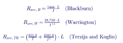
The Warrington formula is often written in US units as R = 8,750·L/I^1.4 with L in feet. The three formulas give results of the same order but not identical, and which one is most conservative depends on the current:
| Arc length | Fault current | Blackburn | Warrington | Terzija-Koglin |
|---|---|---|---|---|
| 3 m | 500 A | 8.66 Ω | 14.34 Ω | 5.19 Ω |
| 3 m | 1,000 A | 4.33 Ω | 5.43 Ω | 2.58 Ω |
| 3 m | 2,000 A | 2.17 Ω | 2.06 Ω | 1.29 Ω |
| 3 m | 5,000 A | 0.87 Ω | 0.57 Ω | 0.51 Ω |
| 3 m | 10,000 A | 0.43 Ω | 0.22 Ω | 0.26 Ω |
| 10 m | 1,000 A | 14.44 Ω | 18.11 Ω | 8.60 Ω |
| 10 m | 2,000 A | 7.22 Ω | 6.86 Ω | 4.29 Ω |
| 10 m | 5,000 A | 2.89 Ω | 1.90 Ω | 1.71 Ω |
| 10 m | 10,000 A | 1.44 Ω | 0.72 Ω | 0.86 Ω |
The Warrington and Blackburn curves cross at about 1,800 A: below that current the Warrington formula gives the highest values, and above it the Blackburn formula does. For setting purposes, use the formula that is most conservative for the fault current range at the relay, typically the minimum current for a remote-end fault under N-1 conditions.
Arc length and stretch. The initial arc length is roughly the flashover distance across the insulator string or the clearance to the structure. Wind, convection and magnetic forces stretch the arc over time. A common US approach based on Warrington's work adds 3·v·t feet to the initial length, where v is wind speed in miles per hour and t is the time in seconds the arc burns before the zone trips. For a time-delayed zone with a 0.5-second delay and a 25-mph wind, the arc can stretch by about 37 feet, or 11 meters. Some transmission owners simplify this by adopting a standard arc length for each zone, for example about 10 meters for a zone with a 0.25-second delay.
Footing resistance. On lines with continuous, grounded shield wires, the fault return path through many parallel tower grounds makes individual footing resistances largely irrelevant. On lines without shield wires, the footing resistance of the faulted structure, often 5 to 20 ohms but sometimes 100 to 200 ohms in rocky or sandy soil, appears in series with the arc and dominates the fault resistance.
Load limit
The right resistive blinder must not encroach on load. Calculate the minimum load impedance at the lowest expected operating voltage, typically 0.85 per unit, and the maximum line loading, often the highest seasonal emergency rating:

For the 230 kV example line with a maximum loading of 1,600 A:

At a load angle of 30 degrees, the load point is 61.1 + j35.3 ohms. Projected onto the resistive axis along the line angle of 82.7 degrees, where a blinder parallel to the line would cross it, the load point corresponds to a resistive reach of about 56.6 ohms. Applying a 20 percent margin gives an upper limit of about 45 ohms primary for the resistive reach. Where the load limit is tighter than the arc requirement, a common rule is to set the resistive reach halfway between the arc resistance requirement and the load limit; where the load limit is below the arc requirement, use the relay's load encroachment logic or a residual current supervision that distinguishes ground faults from balanced load, and accept a compromise.
Remember that relays define resistive reach differently. Some apply it directly to fault resistance. Others apply it to the loop resistance, in which case the fault resistance coverage is reduced by the factor 1 + k0. Always confirm the definition in the relay's instruction manual before converting a resistance requirement into a setting.
The measurement accuracy limit
Small angle errors in CTs, VTs and the relay rotate the measured impedance. For a resistive fault at the remote bus, that rotation can lift or lower the measured point relative to the reactance line. With a very large resistive reach, even a few degrees of error can make a remote-bus fault appear inside Zone 1. Treating the error as a rotation of the fault point by an angle ε about the remote-bus impedance gives the maximum resistive reach that avoids overreach:
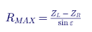
where ZL is the line impedance, ZR is the Zone 1 reactive reach and ε is the total angular error. Typical error contributions are about 0.8 degrees for protection-class CTs, 2 degrees for VTs and 0.2 degrees for the relay, for a total of about 3 degrees. The table shows how the limit depends on both the Zone 1 margin and the error.
| Zone 1 reach | Total angle error | RMAX for ZL = 10 Ω | RMAX as multiple of reactive reach |
|---|---|---|---|
| 80% | 2° | 57.3 Ω | 7.2 |
| 80% | 3° | 38.2 Ω | 4.8 |
| 80% | 5° | 22.9 Ω | 2.9 |
| 85% | 2° | 43.0 Ω | 5.1 |
| 85% | 3° | 28.7 Ω | 3.4 |
| 85% | 5° | 17.2 Ω | 2.0 |
| 90% | 3° | 19.1 Ω | 2.1 |
The often-quoted rule that the resistive reach should not exceed about five times the reactive reach is correct only for the 80 percent, 3-degree case. A Keentel setting calculation computes RMAX for the actual reach, CT and VT accuracy classes and relay, and compares it with the arc and load limits. An alternative is to add a small reactance line tilt, equal to the expected angle error, on top of the non-homogeneity tilt.
Coordinating step-distance Zone 2 for resistive faults
Bolted-fault coordination checks are routine. Resistive-fault coordination is not, and that is where many step-distance coordination failures hide. Several factors cause a backup Zone 2 to lose selectivity with the adjacent line's Zone 1 for resistive faults:
- Different resistive reach definitions. One relay may define resistive reach in terms of fault resistance and another in terms of loop resistance, which differ by the factor 1 + k0.
- Different reactance line tilts. If Zone 2 is tilted differently from the adjacent line's Zone 1, their reactance lines can cross, exposing a region where a resistive fault is in the backup zone but not the primary zone. Use the same tilt for backup and primary zones where possible.
- Different polarizing quantities. Coordinating zones should use the same polarizing method where possible.
- Mho expansion differences. Different relay designs expand their mho circles differently, which matters most when a short line follows a long line.
The reliable way to verify coordination is to apply resistive faults at several locations on adjacent lines in a short-circuit program that models each relay's characteristic, and to check that the primary zone always operates before the backup zone. Where step-distance ground zones cannot provide adequate resistive coverage with secure coordination, use a pilot scheme or inverse-time directional ground overcurrent elements for sensitive ground fault protection.
Setting ground distance in pilot schemes
In POTT, DCB and DCUB schemes, the forward overreaching zone and the reverse blocking zone work together to provide high-speed tripping for the whole line.
- Forward overreaching zone. Often set sensitively, around 150 to 200 percent of the line, so it picks up quickly for any internal fault including resistive faults. It must not be so long that it produces nuisance keying for remote external faults with heavy load or open-pole unbalance.
- Reverse blocking zone. Set to reach farther behind the local terminal than the remote forward zone reaches past it. A common rule sets the local reverse zone reach equal to the remote forward zone reach, so that the line impedance itself acts as the coordination margin. Some utilities subtract the line impedance from the remote forward zone reach when setting the reverse zone; that works for bolted faults but can fail for resistive faults. Verify with resistive faults.
- Current reversal logic. The reverse zone also starts the transient blocking timer that prevents a permissive trip, and blocks echo, during current reversals on parallel lines.
- Ground directional overcurrent. A 67G forward element keyed into the scheme and a more sensitive 67G reverse element extend high-impedance fault coverage beyond what the ground distance zones provide.
Summary of application guidelines
| Application | Ground mho | Ground quadrilateral |
|---|---|---|
| Parallel lines with mutual coupling | Susceptible to overreach and underreach; set from apparent impedance across all parallel line states | Same susceptibility; same method; prefer negative-sequence directional supervision |
| Short lines, weak sources, high SIR | Limited coverage; reduce reach for measurement error | Better resistive coverage, but reactive reach limited by reduced reactance reach |
| CVT transients, CT saturation, inrush | Use relay CVT transient logic with weak sources; dropout extension for overreaching zones | Same; also check false residual currents during inrush |
| Faulted phase selection | Multi-criteria selection; limit phase loop resistive reach near strong sources | Same |
| Underground cables | Preferred if distance is used; pilot or differential schemes preferred overall | Use with caution; resistive reach unreliable |
| Single-pole tripping | Ground mho reliable during open-pole interval | Self-polarized preferred; sequence-polarized must be blocked during open pole |
| Series-compensated lines | Tune with hardware-in-the-loop testing | Tune with hardware-in-the-loop testing |
| Tapped transformers, autotransformers, multi-terminal lines | Consider limited for Zone 2 and outfeed for Zone 1 | Same |
| Zone 1 | About 80 to 85% of the lowest apparent impedance | Reactive reach about 80 to 85%; resistive reach limited by measurement accuracy |
| Long lines | Good coverage and inherent load security | Similar coverage; simpler to use mho |
| Step-distance Zone 2 | At least 120% of the highest apparent impedance; coordinate with adjacent Zone 1 for bolted and resistive faults | Same; match tilt and polarizing to adjacent zones |
| Pilot schemes | Forward zone around 150 to 200%; reverse zone covers remote forward reach | Same; verify reactive and resistive coordination |
How Keentel Engineering helps here: Our setting calculations start with a validated fault study and document every apparent impedance, margin, arc resistance, load limit and accuracy limit behind each zone. We check resistive-fault coordination across relay designs, set pilot forward and reverse zones together for both terminals, and deliver setting files with a calculation record that a reviewer can audit line by line.
15. NERC compliance, testing and documentation
Where ground distance settings meet NERC standards
Several NERC Reliability Standards touch ground distance settings directly or indirectly.
| Standard | Relevance to ground distance |
|---|---|
| PRC-004 | Misoperation identification and corrective action; most ground distance overreach and underreach events are reportable misoperations requiring cause identification and a corrective action plan |
| PRC-027 | Requires a process to coordinate protection systems for faults, including fault current studies and periodic or change-based reviews; ground distance coordination with adjacent zones falls squarely within it |
| PRC-005 | Maintenance and testing intervals for protective relays, instrument transformer inputs, communications and DC supply, all of which affect ground distance performance |
| PRC-023 | Loadability requirements for load-responsive phase protective functions; ground elements are generally outside its scope, but load security of ground zones must still be checked |
| PRC-026 | Relay performance during stable power swings for load-responsive relays identified by the Planning Coordinator |
| PRC-024 and PRC-029 | Ride-through requirements for generating resources; line and tie-line protection at IBR plants must not cause tripping inside the ride-through envelope |
| MOD-032 and MOD-033 | Modeling data and model validation; the short-circuit and dynamic models behind setting studies should be consistent with the data submitted for planning models |
PRC-027 deserves particular attention. Each time a parallel circuit is added, a tap is built, a transformer is replaced or an interconnection is energized, the zero-sequence network changes, and ground distance apparent impedances on nearby lines change with it. A disciplined PRC-027 process that triggers a coordination review on these events, and on significant changes in fault current, is the best defense against ground distance misoperations.
Commissioning tests that catch ground distance errors
Many ground distance misoperations are not setting errors. They are wiring or configuration errors that ordinary checks miss.
- Residual circuit polarity. An in-service load check verifies phase CT polarity and ratio under balanced conditions, but it does not prove the residual circuit. A reversed neutral connection, a missing neutral, or an incorrectly configured residual CT input will not appear until a ground fault. Check the residual circuit with primary injection, or with a deliberate secondary test that produces residual current, before relying on ground elements.
- k0 entry format. Confirm that the k0 entered in the relay matches the relay's definition, especially magnitude and angle versus separate resistive and reactive factors.
- Mutual compensation wiring. If k0M is used, verify the parallel line residual input polarity and ratio.
- State-sequence testing. Test ground zones with prefault, fault and postfault states derived from the fault study, not just with steady-state impedance points, so memory polarization, CVT logic and timers are exercised.
- Event playback. Replay recorded or simulated COMTRADE files of difficult faults, such as resistive faults at the reach point, faults during open-pole intervals and current reversals, through the relay.
- End-to-end pilot tests. Use GPS-synchronized test sets at both terminals to test permissive, blocking, echo and weak-infeed logic with realistic fault quantities.
Documentation that stands up to review
A ground distance setting file should be supported by:
- A written protection philosophy stating zone criteria, margins and the system conditions considered.
- The short-circuit model version, including mutual impedances and tapped sources, and the fault cases studied.
- A calculation record from line constants to secondary settings, including k0, apparent impedances, arc and load limits and accuracy limits.
- Coordination checks with adjacent zones for bolted and resistive faults.
- Commissioning and maintenance test records, including residual circuit verification.
- A change log linking each revision to the system change or event that triggered it.
That package is the evidence that supports PRC-004 cause analysis, PRC-027 coordination reviews and audit questions about how settings were derived.
A ground distance setting workflow
1. Collect data. As-built line routes, conductor and shield wire data, structure types, parallel circuits and their separation, tapped transformers, CT and VT ratios and accuracy classes, relay models and firmware.
2. Build and validate the model. Calculate line constants, including mutual impedances; update the short-circuit model; compare with any available field measurements and recorded faults.
3. Define the cases. Normal topology, N-1 source outages, parallel line states, tap states, series capacitor states, three-terminal configurations and IBR operating modes.
4. Calculate apparent impedances. For remote-bus faults, faults on parallel lines and faults along the line with fault resistance.
5. Set reactive reaches. Zone 1 from the lowest apparent impedance; overreaching zones from the highest; adjust for SIR, CVT transients and series compensation.
6. Set resistive reaches and tilt. From arc and footing requirements, load limits, accuracy limits and non-homogeneity.
7. Choose polarizing and directional elements. Based on mutual coupling, IBR presence, cable sections and single-pole tripping.
8. Coordinate. With adjacent zones for bolted and resistive faults; between pilot forward and reverse zones; with ground overcurrent and breaker failure.
9. Review. Independent peer review of the calculation record.
10. Test and commission. Including residual circuit verification and state-sequence tests.
11. Monitor. Review event reports after every ground fault; re-study when the network changes.
How Keentel Engineering helps here: We support every step of this workflow, from line constants and model validation through setting calculations, peer review, commissioning support and PRC-004 event analysis. Our deliverables are organized to answer the questions auditors and reviewers ask, so clients can show not only what their settings are but why.
Part C — Three Anonymous Case Studies
The following case studies are based on the kinds of ground distance problems Keentel Engineering encounters in practice. Names, locations, equipment and some numbers have been changed or generalized to protect client confidentiality, but the engineering issues, analysis methods and lessons are real.
Case Study 1: Zone 1 overreach during a maintenance outage on a 230 kV double circuit
Background
A transmission owner in the southeastern US operates a 230 kV double-circuit line about 32 miles long between two major substations. Both circuits share lattice towers along the whole route. Each terminal is protected by two microprocessor relays: one running a POTT scheme over fiber with ground mho and ground quadrilateral elements, and one running line current differential with step-distance backup. The ground distance Zone 1 elements were set to 85 percent of the positive-sequence line impedance, with k0 calculated from the line constants. The settings were more than ten years old, dating from a relay replacement project.
The event
Circuit 2 was removed from service for insulator replacement. Following the utility's safety procedures, the crew grounded Circuit 2 at both terminal substations and at the work site. Two days into the outage, a lightning stroke caused an A-phase-to-ground fault on a 230 kV line leaving the remote substation, about 3 miles beyond the remote bus. The Circuit 1 relays at the local substation tripped instantaneously on ground distance Zone 1, along with the correct clearing of the faulted line. With Circuit 2 already out, the trip of Circuit 1 left the remote substation connected to the rest of the system by only two lower-capacity paths, and a 230/115 kV transformer at the remote station briefly exceeded its emergency rating before operators reduced load.
Analysis
Keentel was engaged to perform the PRC-004 cause analysis and recommend corrective actions. We began with the event records from both relays at the tripping terminal. The fault-type selection correctly identified an A-phase-to-ground fault. The measured loop impedance settled at about 79 percent of the circuit's positive-sequence impedance, inside the 85 percent Zone 1 reach, even though the fault was beyond the remote bus.
The utility's short-circuit model included both circuits but did not include their mutual zero-sequence impedance. We calculated line constants from the tower drawings and route data, finding a zero-sequence mutual impedance of about 57 percent of each circuit's zero-sequence self impedance. With the mutual impedance added and Circuit 2 represented as grounded at three points, the model reproduced the recorded relay quantities within 3 percent.
The study then examined all parallel line states for a remote-bus ground fault on Circuit 1:
| Circuit 2 state | Apparent X for remote-bus fault (fraction of line X) |
|---|---|
| In service | 1.27 |
| Open, not grounded | 1.00 |
| Out of service, grounded at both ends | 0.83 |
| Out of service, grounded at both ends and at a midpoint work site | 0.80 |
The study also showed that faults on lines beyond the remote bus, up to about 4 miles away, appeared inside the 85 percent Zone 1 with Circuit 2 grounded.
Solution
Keentel presented three alternatives to the client:
1. Permanently reduce Zone 1 to 85 percent of the lowest apparent impedance, about 68 percent of the line. This was simple but would reduce high-speed coverage during normal operation, when both circuits are in service most of the time.
2. Apply mutual compensation. This was rejected because the grounded circuit's current was not measured by the Circuit 1 relays when Circuit 2's breakers were open, so k0M would not help in the critical condition.
3. Use adaptive setting groups. Bring the Circuit 2 breaker and line disconnect status into the Circuit 1 relays, and switch to a group with a reduced Zone 1 whenever Circuit 2 is out of service, regardless of grounding.
The client chose option 3, combined with a modest reduction of the normal Zone 1 from 85 to 80 percent to allow for line constant uncertainty. The reduced group sets Zone 1 at 64 percent of the line, which is 80 percent of the lowest apparent impedance found with a midpoint work-site ground. Because both terminals have pilot schemes, high-speed clearing of the whole line is preserved in either group. The setting group logic was tested end to end, including loss of the status input, which defaults to the reduced group.
Results and lessons
The corrective action plan was completed within the PRC-004 timeline. The client then asked Keentel to screen its other double-circuit and shared-corridor lines. Of 27 lines screened, 9 had mutual coupling that was missing or incomplete in the short-circuit model, and 4 had Zone 1 settings that would overreach with a parallel line grounded.
- Mutual impedance must be in the short-circuit model. A model without it is not suitable for ground protection settings.
- The grounded parallel line is a normal operating condition and must be studied.
- k0M does not protect against overreach when the parallel line is out of service.
- Status-based setting groups recover coverage, but their failure mode must default to the secure group.
Case Study 2: Ground element behavior at a 345 kV solar and storage interconnection
Background
A developer in the Midwest was building a 300 MW solar plant with a 150 MW battery energy storage system, connected through two 34.5/345 kV main power transformers (wye-grounded on the 345 kV side, delta on the 34.5 kV side) and a 14-mile 345 kV generator tie line to a utility switching station. The utility required line current differential as primary protection and a POTT scheme with ground distance and directional ground overcurrent elements as secondary protection. The developer's original relay settings, prepared early in the project, used negative-sequence-polarized ground quadrilateral elements and negative-sequence directional supervision at both ends of the tie line.
The concern
During the interconnection review, the utility asked for demonstration that the plant-end relays would operate correctly for ground faults on the tie line, given the inverters' fault current characteristics. The inverter manufacturer's documentation showed that the inverters limited fault current to about 1.1 per unit and that the negative-sequence current injection mode was configurable. The project team was not sure which mode would be enabled in the final commissioning.
Analysis
Keentel built short-circuit models of the plant using the inverter manufacturer's voltage-dependent current source data and EMT models using the vendor-supplied inverter models, validated against the plant's IEEE 2800 performance documentation. We simulated A-phase-to-ground faults along the tie line with fault resistances from 0 to 30 ohms, in two inverter modes: with negative-sequence injection enabled per the standard and with it suppressed.
Key findings at the plant-end relay:
| Quantity | Negative-sequence injection enabled | Negative-sequence injection suppressed |
|---|---|---|
| Phase current, bolted fault at utility end | About 1.1 per unit of plant rating, controlled angle | About 1.1 per unit of plant rating, mostly positive sequence |
| Negative-sequence current | Moderate, inductive-like angle | Near zero |
| Zero-sequence current | Large, supplied by the wye-grounded transformers | Large, supplied by the wye-grounded transformers |
| Negative-sequence directional element | Correct, with margin | Unreliable: quantities below threshold for some faults |
| Negative-sequence-polarized quadrilateral | Correct for bolted faults, reactance error up to 20% for 20-ohm faults | Unreliable |
| Ground mho, memory-polarized | Correct | Correct |
| Zero-sequence directional element | Correct | Correct |
| Fault-type selection | Correct | Wrong loop selected in 2 of 24 resistive fault cases during the first cycle |
The zero-sequence quantities at the plant end were dominated by the main power transformers and were large and stable regardless of inverter mode. The negative-sequence quantities depended entirely on the inverter controls.
Solution
Keentel recommended and the developer and utility agreed:
- Change the plant-end ground quadrilateral elements to zero-sequence current polarization, with a tilt calculated from the zero-sequence network, which the inverters do not affect.
- Change the plant-end directional supervision to zero-sequence voltage polarization with current polarization from the main power transformer neutral CT as a backup. Mutual coupling was not significant on this route, which was confirmed by a corridor review.
- Enable the relay's voltage-based fault-type selection supervision.
- Retain ground mho elements as the main overreaching pilot elements, since they performed correctly in every case.
- Add weak-infeed echo at the plant end, so that the utility end trips at high speed even for resistive faults near the plant, where the plant end might not key on its own.
- Require, in the commissioning plan, confirmation of the final inverter negative-sequence mode and a repeat of the critical simulations if it differed from the studied mode.
Results and lessons
The revised settings were verified with hardware-in-the-loop playback of 120 EMT cases through the actual relays. All internal faults were cleared at high speed by at least one scheme, and no external fault produced a trip. The utility accepted the protection package without further comments.
- At IBR terminals, zero-sequence quantities from the main power transformer are usually more dependable than negative-sequence quantities from the inverters.
- Inverter operating modes are settings too. Protection studies must state the mode they assume, and commissioning must confirm it.
- EMT simulation is needed to evaluate fault-type selection and directional decisions during the first cycles of an IBR fault.
Case Study 3: A data center tap changes the ground protection of a 138 kV line
Background
A transmission utility in the south-central US received an interconnection request for a large data center campus. The initial phase would connect two 138/34.5 kV, 80 MVA transformers, wye-grounded on the 138 kV side and delta on the 34.5 kV side, tapped from an existing 26-mile 138 kV line about 9 miles from Bus A. A switching station with breakers was planned for a later phase; the first phase would use a breakerless tap with high-side circuit switchers to meet the customer's energization schedule. The existing line had step-distance ground mho elements and directional ground overcurrent protection at both ends, with no pilot channel.
The concern
The utility's planning study confirmed thermal and voltage adequacy, but the protection review identified that the two new wye-grounded transformers would become a strong zero-sequence source in the middle of the line. Keentel was retained to evaluate the effect on the existing line protection and on adjacent lines, and to recommend changes.
Analysis
We updated the short-circuit model with the new transformers, their zero-sequence impedances from the transformer test reports, and the tap location. For a ground fault at Bus B, with both data center transformers in service:
| Quantity at Bus A relay | Without tap | With tap |
|---|---|---|
| Residual current 3I0 | 2,850 A | 1,880 A |
| Apparent ground impedance (fraction of line Z1) | 1.00 | 1.31 |
| Existing Zone 2 reach (fraction of line Z1) | 1.30 | 1.30 |
| Zone 2 sees bolted Bus B ground fault? | Yes | No |
The existing Zone 2 ground mho at Bus A, set to 130 percent of the line, no longer reached the remote bus for ground faults. The same effect occurred at Bus B. The directional ground overcurrent elements still detected the faults, but their time delays, coordinated with downstream ground overcurrent relays, gave clearing times of 0.9 to 1.4 seconds for faults near the remote ends of the line, which exceeded the utility's planning criteria for that line.
We also examined reach-through. With Bus B open and the tap fed from Bus A, a ground fault on the 34.5 kV side of the data center transformers cannot produce zero-sequence current on the 138 kV side, because of the delta windings, and phase-to-phase faults on the 34.5 kV side appeared well outside the phase Zone 1. Reach-through was not a concern for this configuration, but we documented it because a future change to wye-grounded/wye-grounded transformers with a delta tertiary would change the answer.
Solution
Keentel recommended a two-stage solution
Stage 1, at energization of the tap:
- Increase Zone 2 ground reach at both terminals to 125 percent of the highest apparent impedance with the tap in service, about 164 percent of the line, and increase the Zone 2 time delay from 20 to 30 cycles to restore coordination with the adjacent lines' Zone 2, where the new reach overlapped them.
- Add a sensitive definite-time directional ground overcurrent element as a supplement for high-resistance faults, coordinated with the new Zone 2.
- Leave Zone 1 at 80 percent of the line impedance with the tap disconnected, because the tap makes Zone 1 underreach, which is secure.
- Document the change under the utility's PRC-027 process and update the coordination database.
Stage 2, with the switching station:
- Install fiber and convert the line into two line sections with line current differential and POTT backup, which removes the infeed problem entirely by placing breakers at the tap.
Results and lessons
Stage 1 was implemented before the first data center transformer was energized. Event reports from two subsequent ground faults on the line, both cleared by the revised Zone 2 within the expected times, matched the study within 5 percent.
- A new grounded transformer tap anywhere on a line changes the ground distance reach of every terminal of that line, and sometimes of adjacent lines.
- Large-load interconnection studies need a protection review, not just thermal and voltage analysis.
- Interim configurations, such as breakerless taps used to meet schedules, need their own protection study.
- Keeping the transformer winding configuration in the study record matters, because a later equipment change can turn a secure configuration into a reach-through problem.
Part D — Technical FAQ: 30 Questions on Ground Distance Protection
Fundamentals
1. Why does a ground distance element need k0 when a phase distance element does not?
A phase loop measures the difference between two phase voltages divided by the difference between two phase currents. In that difference the zero-sequence components cancel, and the ratio equals the positive-sequence impedance to the fault. A ground loop measures one phase voltage, and the voltage drop along the line for a ground fault includes the zero-sequence drop, which is governed by Z0L rather than Z1L. Adding k0·3I0 to the phase current scales the residual current so that the ratio again equals m·Z1L. Without k0, a ground element would measure (2Z1L + Z0L)/3 per unit length for a radial fault, which for a typical overhead line with Z0/Z1 near 3 is about 67 percent higher than Z1L, and every ground zone would underreach badly.
2. What is a typical value of k0 for US overhead transmission lines?
For overhead lines with shield wires, Z0L/Z1L is typically 2.5 to 3.5, which gives a k0 magnitude of about 0.5 to 0.85. The angle is usually small and negative, from about −2 to −15 degrees, because the zero-sequence impedance angle is a few degrees lower than the positive-sequence angle. Lines without shield wires, or with high earth resistivity, tend toward the upper end of the range. Values well outside this range, for example a k0 magnitude above 1.2 or a large positive angle, are worth double-checking, unless the circuit includes cable sections or unusual construction.
3. Should k0 be calculated from total line impedances or per-mile values?
For a homogeneous line, the result is the same. For a line with sections of different construction, such as a change from single-circuit to double-circuit towers, a different conductor, or a cable section, calculate the total Z1L and Z0L by adding the section impedances and compute k0 from the totals. This makes the ground element measure correctly for a remote-bus fault. Faults inside the line will then have small errors that depend on how the sections differ, and those errors should be checked against the Zone 1 margin.
4. Why do some relays ask for RE/RL and XE/XL instead of k0?
Those relays apply the zero-sequence compensation separately to the resistive and reactive parts of the loop. RE/RL equals (R0L − R1L)/(3·R1L) and XE/XL equals (X0L − X1L)/(3·X1L). Because the zero-sequence resistance of an overhead line is much larger relative to its positive-sequence resistance than the reactances are to each other, RE/RL is usually much larger than XE/XL. In Worked Example 1, RE/RL is 1.17 while XE/XL is 0.69. Entering the complex k0 magnitude into both fields is a common and significant mistake.
5. How does memory polarization affect the reach of a ground mho element?
Memory polarization does not change the reach along the line angle; the expanded circle still passes through the reach point. It enlarges the circle toward the source, so that for forward faults the characteristic extends from the reach point back toward −ZS. This adds resistive coverage, especially for faults close to the relay and on weak systems where ZS is large. For reverse faults the characteristic shifts away from the origin, which improves directional security. Once the memory decays, the characteristic shrinks back toward the self-polarized circle, so the extra coverage is temporary for sustained faults unless the relay blends present and memory voltage.
6. Why is a ground quadrilateral element sometimes slower than a ground mho element?
A quadrilateral zone requires four separate comparators, for the reactance line, two resistive blinders and the directional line, to agree. Its output is only as fast as the slowest of the four. For faults near any boundary, at least one comparator is close to its decision threshold, where filtering and security counters slow it down. A mho element uses a single comparison. Modern relays reduce this difference with fast filtering and parallel processing, but the principle explains why some quadrilateral implementations are slightly slower near the zone boundaries.
Mutual coupling and network effects
7. How large can the mutual coupling error be in practice?
On a double-circuit line with a mutual impedance of about 55 to 60 percent of the zero-sequence self impedance, the apparent impedance for a remote-bus ground fault can be 25 to 30 percent higher than the line impedance with the parallel circuit in service, and 15 to 20 percent lower with the parallel circuit out of service and grounded at both ends. In Worked Example 4, the range is 0.81 to 1.29 times the true value. Errors of this size are larger than the typical margins in Zone 1 and Zone 2 settings, which is why mutual coupling must be studied explicitly.
8. When should k0M mutual compensation be used?
Use k0M when the parallel line's residual current is reliably available to the relay, when the coupling error is large enough to compromise the overreaching zones, and when the relay provides supervision that disables mutual compensation for faults on the parallel line. It is most useful for extending overreaching zones and improving fault location accuracy. It does not help when the parallel line is out of service and grounded with its breakers open, because the induced current is not measured. Applying k0M to Zone 1 requires a study showing that faults on the parallel line near the remote bus do not cause overreach.
9. Can lines at different voltages be mutually coupled?
Yes. Zero-sequence coupling depends on geometry and earth return, not voltage. A 69 kV line under a 230 kV line, or a 115 kV circuit on the lower arms of a 345 kV double-circuit tower, can be strongly coupled. The lower-voltage circuit's relays are usually affected more, because their own fault currents are smaller while the induced voltage from a fault on the higher-voltage circuit can be large. These cases are often missed because the circuits belong to different planning areas or owners.
10. Why is negative-sequence polarization preferred for directional elements on coupled lines?
Zero-sequence mutual coupling induces zero-sequence voltage in the healthy circuit and can drive zero-sequence current in directions that do not reflect the fault location relative to that circuit. A zero-sequence voltage-polarized directional element on the healthy circuit can therefore declare a forward fault when the fault is on the parallel circuit. Negative-sequence coupling between circuits is small, so negative-sequence directional elements are much less affected. The exception is where negative-sequence quantities are small or unreliable, such as near inverter-based resources.
11. What is current reversal, and how do ground distance settings interact with it?
When a fault on one of two parallel lines is cleared sequentially, the opening of the first breaker can reverse the current direction in the healthy parallel line. Relays on the healthy line that had seen a reverse fault suddenly see a forward fault, and vice versa. In a POTT scheme, the healthy line can trip if one terminal's forward element picks up before the other terminal's forward element drops out. Transient blocking logic, started by the reverse zone, holds off permissive tripping for a short time after a reverse fault is detected. Ground distance settings support this by making the reverse zone reach beyond everything the remote forward zone can see, so the reverse zone always picks up when needed.
12. How does a tapped wye-grounded transformer affect ground distance relays at the line terminals?
The tapped transformer provides a zero-sequence path to ground at the tap. For a ground fault beyond the tap, it supplies part of the fault's zero-sequence current, so the terminal relays see less residual current than the fault draws. Their compensated loop current is reduced relative to the voltage, and they measure a higher apparent impedance, so ground zones underreach. In Worked Example 9, a 50 MVA tap at the midpoint of a 138 kV line raised the apparent impedance for a remote-bus fault by 26 percent. Overreaching zones must be extended to cover it, while Zone 1 can remain based on the line impedance without the tap.
Instrument transformers and measurement
13. Why do CVT transients mainly affect Zone 1?
The CVT transient lasts roughly one to two cycles. During that time the filtered voltage can be lower than the true voltage, making the measured impedance smaller than it should be. Zone 1 trips without intentional delay, so a brief excursion into the zone can cause a trip. Zone 2 and Zone 3 have time delays much longer than the transient, so the measurement has recovered before their timers expire. Pilot overreaching zones are not a security concern either, because they are designed to overreach and are supervised by the other terminal.
14. Does CT saturation make ground distance elements overreach?
Usually not. Saturation reduces the measured current magnitude, which increases the computed impedance and causes underreach. The main risk is reduced dependability: slower operation for faults near the zone boundary and possible dropout of time-delayed zones. Saturation also shifts the current phase angle, which can affect directional decisions and fault-type selection, and unequal saturation of phase CTs produces false residual current. These secondary effects can occasionally threaten security, especially for sensitive ground overcurrent elements during transformer energization.
15. How should CTs be sized for ground distance applications?
The governing condition is usually the overreaching pilot zone or Zone 2 for a fault at the remote end of the line, because that element must operate dependably and quickly. A widely used criterion permits a burden up to 6·VK/((X/R + 1)·ISF), which allows some saturation for close-in faults while protecting the overreaching zone's performance. The stricter IEEE C37.110 saturation-free criterion, VS ≥ (1 + X/R)·IF·ZB, is often impractical for high X/R transmission faults. Use the CT at full ratio, minimize lead burden, and consult the relay maker's guidance for the specific relay.
16. What SIR makes a line "short" for protection purposes?
IEEE C37.113 classifies lines with an SIR greater than 4 as short, between 0.5 and 4 as medium, and less than 0.5 as long. The classification depends on the source behind the relay as well as the line. Because the source impedance increases when generators or transformers are out of service, the N-1 SIR is often several times the normal SIR. Calculate SIR from a fault study using the relay voltage for a remote-bus fault, separately for ground and phase faults.
17. How much should Zone 1 be reduced on a high-SIR line?
The required reduction depends on the measurement error and the SIR. As a rough guide, a fixed voltage error of δ (per unit of nominal) produces an impedance error of about δ·(1 + SIR). With a 1 percent total error, the impedance error is 5 percent at SIR 4, 11 percent at SIR 10 and 31 percent at SIR 30. Zone 1 must leave a margin larger than that error plus allowances for line constant and CVT transient errors. At very high SIRs no secure Zone 1 may exist, and the line should rely on pilot protection, with Zone 1 disabled or delayed.
Quadrilateral settings
18. How do I choose the resistive reach of a ground quadrilateral element?
Start with the fault resistance you need to cover: arc resistance from an appropriate formula with arc stretch for the zone's time delay, plus tower footing resistance if the line has no shield wire, multiplied by the infeed factor at the relay. Then calculate the upper limits: the minimum load impedance at 0.85 per unit voltage with a margin of at least 20 percent, projected along the line angle; and the accuracy limit RMAX = (ZL − ZR)/sin ε. Set the reach between the coverage requirement and the lower of the two upper limits, often halfway between them. Confirm whether the relay defines resistive reach in terms of fault resistance or loop resistance.
19. What is the non-homogeneity tilt, and when do I need it?
The tilt is an angular correction to the quadrilateral reactance line. With fault resistance, the voltage across the fault resistance is in phase with the total fault current, which differs in phase from the current measured at the relay when the system is non-homogeneous or carries load. The difference rotates the apparent fault resistance and makes the reactance element overreach or underreach. The tilt equals the angle between the fault current and the polarizing current at the reach point. It is needed whenever a quadrilateral has a large resistive reach and the sources and line have different impedance angles, which is most of the time.
20. Which polarizing current should I choose for the quadrilateral reactance line?
Negative-sequence current is the best general choice on conventional systems because the negative-sequence network is the most homogeneous and is unaffected by load and zero-sequence mutual coupling, so the required tilt is small. Zero-sequence current is a good choice where strong local zero-sequence sources exist and mutual coupling is absent, and it is often the most reliable choice at IBR terminals. Loop current polarization is the most dependable during single-pole open intervals and for any fault type, but its tilt depends on load and is difficult to set securely. Whichever is chosen, use the same polarizing method for zones that must coordinate.
21. Is the "five times the reactive reach" rule for resistive reach reliable?
No, not as a general rule. It comes from one set of conditions: a Zone 1 at 80 percent of the line and a total angular error of 3 degrees. The accuracy limit depends on the Zone 1 margin and the actual instrument transformer accuracy. At 85 percent reach and 3 degrees of error the limit is about 3.4 times the reactive reach; at 5 degrees it is about 2 times. Calculate RMAX for the actual settings and equipment.
22. Which arc resistance formula should I use?
All three common formulas, from Blackburn, Warrington, and Terzija and Koglin, give values of the same order. Which one is most conservative depends on the fault current: Warrington gives the highest values below about 1,800 A, and Blackburn gives the highest values above that. For setting a resistive reach, use the formula that gives the largest resistance in the current range at the relay, typically the minimum remote-end fault current under N-1 conditions, and include arc stretch for the zone's time delay. Remember that arc resistance is often small compared with tree contact or footing resistance, which may govern instead.
Special applications
23. Should ground distance protection be used on underground cables?
It can be used, but with caution, and usually not as the primary protection. Cable zero-sequence impedance depends on the ground return path, which changes with fault location, sheath bonding and nearby metallic paths, so no single k0 is correct for all faults. In Worked Example 7, a wrong k0 choice produced measurements from 31 percent to 283 percent of the true value. Line current differential is the preferred primary protection for cables. If ground distance is used, choose the Zone 1 k0 that cannot overreach for any return path, the pilot overreaching zone k0 that cannot underreach, prefer mho elements and negative-sequence polarizing, and base settings on phase-domain cable studies.
24. How do single-pole trip schemes affect ground distance relays on a parallel line?
During the single-pole dead time on the faulted line, the open phase's load transfers to the parallel line, which then carries significant zero- and negative-sequence current. Long-reaching or sensitive ground elements on the parallel line can pick up under heavy load. Set their time delays longer than the faulted line's single-pole dead time plus margin, or block them during that interval using open-pole information, and check sequence-polarized elements and sequence directional elements for incorrect decisions.
25. Why can a fault on a series-compensated line appear to be behind the relay?
When the series capacitor is between the relay's VT and the fault, and the capacitor reactance is larger than the line reactance to the fault, the net reactance is capacitive. The relay voltage reverses relative to the current, which is voltage inversion, and a simple directional or distance element sees a reverse fault. Memory polarization and directional logic designed for series compensation preserve correct direction for the duration of the memory. In Worked Example 8, with a 50 percent capacitor at the relay end, faults on the first half of the line show negative reactance.
26. How do inverter-based resources affect ground distance protection?
IBRs supply limited fault current, and its sequence content and angle are determined by their control systems. Older or non-compliant inverters may supply little negative-sequence current, which can upset negative-sequence directional elements, negative-sequence-polarized quadrilateral elements and fault-type selection. The plant's wye-grounded main power transformer is usually a strong zero-sequence source, so ground distance and zero-sequence-based elements often remain dependable. IEEE 2800-2022 requires negative-sequence current injection during unbalanced faults, which improves the situation for new plants, but the actual inverter mode must be confirmed. Use EMT studies with manufacturer models for critical settings.
27. How do I handle a three-terminal line?
Infeed from the third terminal makes faults beyond the tap appear farther away, so overreaching zones at each terminal must reach at least 125 percent of the apparent impedance to the farthest terminal with all sources in service. Outfeed can make internal faults appear closer or prevent overreaching zones from seeing them, so Zone 1 must consider outfeed and pilot dependability must be checked with outfeed present. Short and long legs often require different settings at each terminal. Line current differential protection simplifies three-terminal lines considerably and is widely used at 230 kV and above.
Compliance and practice
28. Are ground distance elements subject to PRC-023 loadability requirements?
PRC-023 addresses load-responsive phase protective functions, such as phase distance, phase overcurrent and certain pilot elements, and ground elements are generally outside its scope. That does not mean load can be ignored. Ground quadrilateral resistive blinders must still be set clear of the minimum load impedance, and long ground zones must remain secure against unbalanced load and open-pole unbalance on parallel lines. Document the load security check alongside the PRC-023 calculations for the phase elements.
29. How often should ground distance settings be reviewed?
At a minimum, whenever the zero-sequence network near the line changes: a new parallel line, a new tap or transformer, a transformer replacement with a different winding configuration, a new interconnection, a series capacitor addition, or a cable section. PRC-027 requires a coordination process with either periodic studies at intervals not exceeding six calendar years or comparison of fault currents against a baseline with re-study when they change significantly. Ground faults that occur on the line are also opportunities: review the event reports and compare the measured apparent impedances with the study.
30. What is the most common root cause of ground distance misoperations?
In Keentel's experience, the most common root causes are incomplete short-circuit models, especially missing or wrong mutual impedances and missing tapped ground sources; wrong k0 entry, such as entering the complex k0 magnitude into separate resistive and reactive fields; unverified residual circuits whose polarity or connection was never proven by a ground current test; and settings that were not re-studied after a network change. Each of these is preventable with a validated model, a careful calculation record, residual circuit commissioning tests and a disciplined change-review process.
How Keentel Engineering Helps
Keentel Engineering is a US power system engineering firm that plans, studies, designs and commissions electrical systems for utilities, transmission owners, independent power producers, large-load customers such as data centers, industrial plants and campuses, from 4 kV distribution to 765 kV transmission. Protection and control engineering is one of our core disciplines. For transmission line protection, and ground distance protection in particular, our services include:
- Transmission line protection setting calculations: complete setting packages for ground and phase distance, directional ground overcurrent, line current differential, pilot schemes (POTT, DCB, DCUB), breaker failure, reclosing and single-pole tripping, with a documented calculation record from line constants to secondary settings.
- Line constants and mutual coupling studies: calculation of positive-, zero- and mutual-sequence impedances from as-built route data, structure types, conductors, shield wires and earth resistivity, including corridor-wide coupling between circuits of different voltages and owners.
- Short-circuit model development and validation: building and correcting fault models with mutual impedances, tapped transformers, autotransformers, three-terminal lines and IBR fault current models, and validating them against recorded events.
- Protection coordination studies and PRC-027 programs: system-wide coordination reviews for bolted and resistive faults, fault current baseline tracking and change-triggered re-studies that meet NERC PRC-027 requirements.
- Misoperation analysis and PRC-004 support: event report and oscillography analysis, root cause identification, model reconstruction, and corrective action plans with documented verification.
- IBR and large-load interconnection protection: protection studies for solar, wind, battery storage and data center interconnections at 69 kV through 345 kV and above, including EMT simulation of inverter fault behavior consistent with IEEE 2800 performance, and coordination with the host utility's requirements.
- Series-compensated and complex line studies: zone-of-impact analysis, EMT models with MOV and bypass logic, preliminary settings and hardware-in-the-loop test support.
- Underground and hybrid cable protection: phase-domain cable modeling with sheath bonding, compensated loop impedance studies and selection between ground distance, negative-sequence directional comparison and line current differential.
- Instrument transformer application: CT sizing and saturation studies to IEEE C37.110 methods, CVT transient assessment, SIR studies and specification of CT and CVT ratings for new substations.
- Relay testing and commissioning: test plans, state-sequence and COMTRADE playback test files, end-to-end pilot scheme testing, residual circuit verification and commissioning witness services.
- PRC-005 maintenance program support: protection system maintenance program development, test procedures and documentation reviews.
- Substation design: physical and protection and control design for transmission substations, switching stations and interconnection substations, from one-lines and three-lines to panel layouts and wiring.
- Owner's engineer and peer review: independent review of protection philosophies, setting packages and interconnection protection designs prepared by others.
- Training: in-house training for protection engineers and technicians on ground distance, mutual coupling, quadrilateral settings and event analysis.
Why Clients Choose Keentel
- Protection expertise backed by system studies: our protection engineers work alongside our short-circuit, dynamic and EMT modeling teams, so settings are based on models we trust and can explain.
- Independent advice: we are not tied to any relay or equipment supplier, so our recommendations follow the engineering and the client's philosophy.
- US standards fluency: daily work with NERC PRC and MOD standards, IEEE C37 protection guides, IEEE 2800, NESC and FERC interconnection requirements.
- Auditable deliverables: every setting traces back to a documented study, case and margin, organized for peer review, PRC-004 analysis and PRC-027 records.
- Field experience: the engineers who calculate settings also support testing, commissioning and post-event analysis.
- Full voltage range: from 4.16 kV plant distribution to 765 kV transmission substations, including the interconnection facilities that connect new generation and large loads to the grid.
Talk to an Engineer
Reviewing ground distance settings on parallel lines, interconnecting an inverter-based plant or a large load, or investigating a ground fault misoperation? Keentel Engineering can review your system and deliver a documented, defensible answer.
- Phone: (813) 389-7871
- Email: contact@keentelengineering.com
- Book a 15-minute call: calendly.com/keentel-engineering/15min
References
- IEEE Std C37.113-2015, IEEE Guide for Protective Relay Applications to Transmission Lines.
- IEEE Std C37.110, IEEE Guide for the Application of Current Transformers Used for Protective Relaying Purposes.
- IEEE Std C37.116, IEEE Guide for Protective Relay Application to Transmission-Line Series Capacitor Banks.
- IEEE Std C37.104, IEEE Guide for Automatic Reclosing on AC Distribution and Transmission Lines.
- IEEE Std C37.114, IEEE Guide for Determining Fault Location on AC Transmission and Distribution Lines.
- IEEE Std C37.2, IEEE Standard for Electrical Power System Device Function Numbers, Acronyms, and Contact Designations.
- IEEE Std C57.13, IEEE Standard Requirements for Instrument Transformers.
- IEEE Std 2800-2022, IEEE Standard for Interconnection and Interoperability of Inverter-Based Resources Interconnecting with Associated Transmission Electric Power Systems.
- IEEE Std 80, IEEE Guide for Safety in AC Substation Grounding.
- NERC Reliability Standards PRC-004, PRC-005, PRC-023, PRC-024, PRC-026, PRC-027, PRC-029, MOD-032 and MOD-033, current effective versions.
- J. L. Blackburn and T. J. Domin, Protective Relaying: Principles and Applications, CRC Press.
- S. H. Horowitz and A. G. Phadke, Power System Relaying, Wiley.
- P. M. Anderson, Power System Protection, IEEE Press and McGraw-Hill.
- A. R. van C. Warrington, "Reactance Relays Negligibly Affected by Arc Impedance," Electrical World, September 1931.
- V. V. Terzija and H. J. Koglin, "A New Approach to Arc Resistance Calculation," Electrical Engineering, vol. 83, 2001.
- L. M. Wedepohl, "Polarised Mho Distance Relay: New Approach to the Analysis of Practical Characteristics," Proceedings of the IEE, vol. 112, no. 3, 1965.
- Keentel Engineering, companion technical blogs: IBR unbalanced faults and negative-sequence current, 50N/51N ground overcurrent protection, SLG versus three-phase faults, zero-sequence and dq0 transformation, weak-grid inverter stability, PRC-030-1 IBR event mitigation, PRC-028-1 IBR disturbance monitoring, MOD-033 model validation, protection relay SAT for MV switchgear, and grounding system testing.
Disclaimer
This article is for general technical information only. Worked examples and case studies use illustrative system data and simplified assumptions; they are not settings for any specific line or relay. Relay designs differ in their definitions of reach, compensation, polarizing and resistive coverage, so always confirm settings against the relay manufacturer's instruction manual and application guidance. Standards are cited as of publication and may be revised. Protective relay settings must be calculated, reviewed, tested and approved by qualified engineers using validated, site-specific models and data, in accordance with the applicable NERC Reliability Standards and the transmission owner's protection philosophy.
© Keentel Engineering
| Office | Address | Phone |
|---|---|---|
| Head Office — Tampa | 400 N Ashley Dr STE #2600, Tampa FL 33602 | (813) 389-7871 |
| Austin | 5900 Balcones Drive STE 100, Austin TX 78731 | (512) 591-0752 |
| Sacramento | 1401 21st St Ste R, Sacramento CA 95811 | (916) 913-4524 |
| Baltimore | 306 W Redwood St STE 200, Baltimore MD 21201 | (410) 225-2181 |


About the Author:
Sandip "Sonny" R. Patel, P.E.
IEEE Senior Member · Founder & CEO, Keentel Engineering
In 1995, Sonny Patel earned his Electrical Engineering degree from the University of Illinois. But degrees don't build legacies — action does.
For three decades, he has worked the power industry from every side of the table: 16 years as a utility engineer at Exelon/Commonwealth Edison; generation leadership across hydroelectric, industrial steam turbine, and a 9 GW renewable fleet; NERC Regional Entity Senior Compliance Engineer and Audit Team Lead, auditing some of the nation's largest utilities; and testing and commissioning lead on equipment up to 765 kV — the very top of the North American grid.Utility. Generator. Regulator. Consultant. Few engineers have seen all four seats. Fewer still have sat in them.
His experience spans nuclear, hydro, conventional generation, renewables, oil and gas, mining — and today's data centers, where he is authoring a three-book series on data center design. He is a Licensed Professional Engineer in six states and a Licensed Electrical Contractor in Florida (Unlimited EC) — he doesn't just design the work; he's qualified to stand behind its execution.Today, as Founder and CEO of Keentel Engineering, Sonny leads a nationwide team of engineers delivering substation design, power system studies, NERC compliance, and commissioning — done right, coast to coast.Three decades. Every side of the table. One standard: accountable engineering.
Services

Let's Discuss Your Project
Let's book a call to discuss your electrical engineering project that we can help you with.
About the Author:
Sandip "Sonny" R. Patel, P.E.
IEEE Senior Member · Founder & CEO, Keentel Engineering
In 1995, Sonny Patel earned his Electrical Engineering degree from the University of Illinois. But degrees don't build legacies — action does.
For three decades, he has worked the power industry from every side of the table: 16 years as a utility engineer at Exelon/Commonwealth Edison; generation leadership across hydroelectric, industrial steam turbine, and a 9 GW renewable fleet; NERC Regional Entity Senior Compliance Engineer and Audit Team Lead, auditing some of the nation's largest utilities; and testing and commissioning lead on equipment up to 765 kV — the very top of the North American grid.
Utility. Generator. Regulator. Consultant. Few engineers have seen all four seats. Fewer still have sat in them.
His experience spans nuclear, hydro, conventional generation, renewables, oil and gas, mining — and today's data centers, where he is authoring a three-book series on data center design. He is a Licensed Professional Engineer in six states and a Licensed Electrical Contractor in Florida (Unlimited EC) — he doesn't just design the work; he's qualified to stand behind its execution.
Today, as Founder and CEO of Keentel Engineering, Sonny leads a nationwide team of engineers delivering substation design, power system studies, NERC compliance, and commissioning — done right, coast to coast.Three decades. Every side of the table. One standard: accountable engineering.
Leave a Comment
Thank you for contacting us.
We will get back to you as soon as possible.
We will get back to you as soon as possible.
Oops, there was an error sending your message.
Please try again later.
Please try again later.
Related Posts
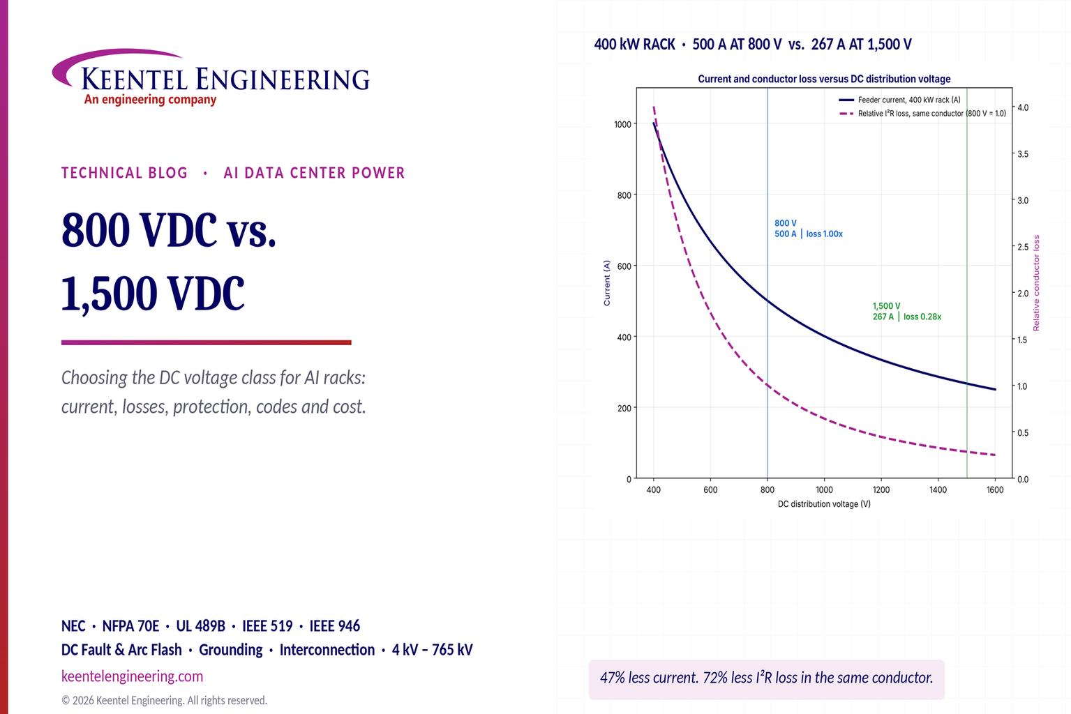
By SANDIP R PATEL
•
November 12, 2026
Compare 800 VDC vs. 1500 VDC for AI data centers. Explore efficiency, copper savings, DC protection, safety and power distribution with Keentel Engineering.
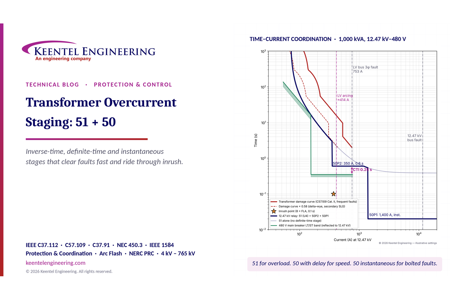
By SANDIP R PATEL
•
November 12, 2026
Learn transformer overcurrent protection using 50/51 relay stages, inverse-time curves, inrush checks, fault coordination and arc-flash mitigation.
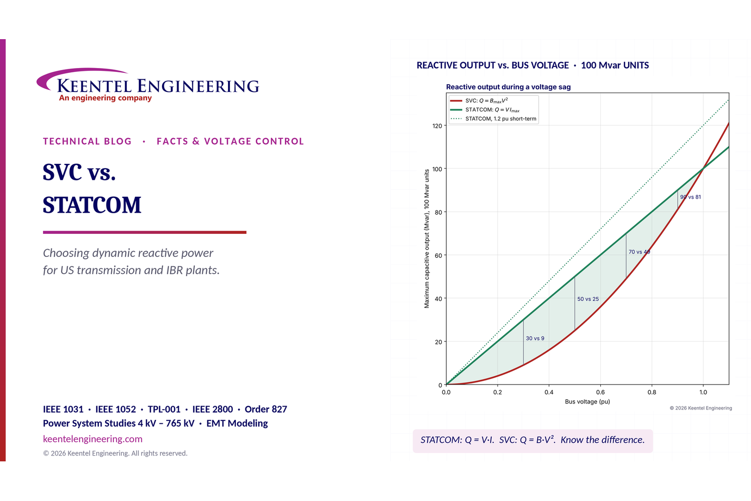
By SANDIP R PATEL
•
November 12, 2026
Compare SVC vs. STATCOM for dynamic reactive power compensation, voltage stability, weak grids, response time, harmonics and transmission system design.
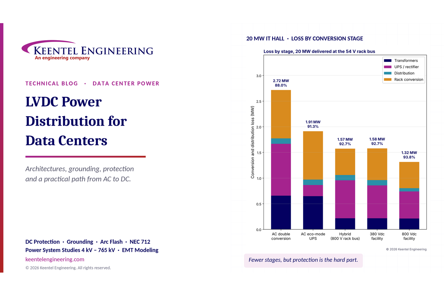
By SANDIP R PATEL
•
November 11, 2026
Explore LVDC power distribution for data centers, including 380V vs 800V DC, architecture, grounding, protection, UPS, energy efficiency and safety standards.
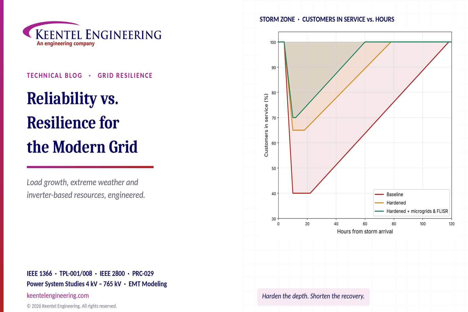
By SANDIP R PATEL
•
November 11, 2026
Explore grid reliability vs. resilience, extreme weather planning, outage recovery, IEEE 1366 metrics, microgrids and IBR challenges with Keentel Engineering.
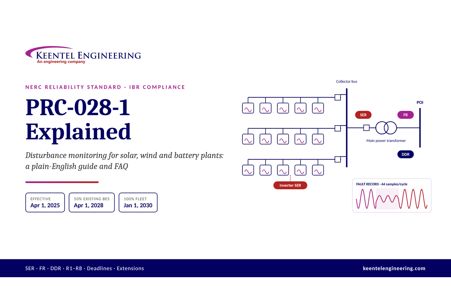
By SANDIP R PATEL
•
November 10, 2026
Learn NERC PRC-028-1 requirements for solar, wind and BESS, including disturbance monitoring, recording standards, deadlines and compliance steps from Keentel.
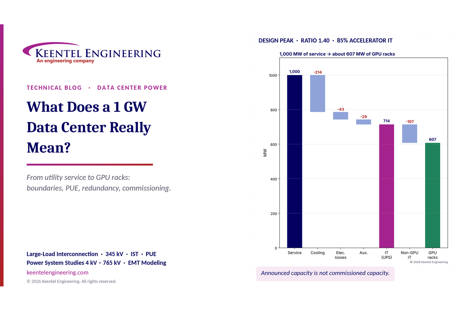
By SANDIP R PATEL
•
November 8, 2026
What does a 1 GW data center mean? Explore power capacity, PUE, GPU racks, grid interconnection and commissioning with Keentel Engineering's expert guide.
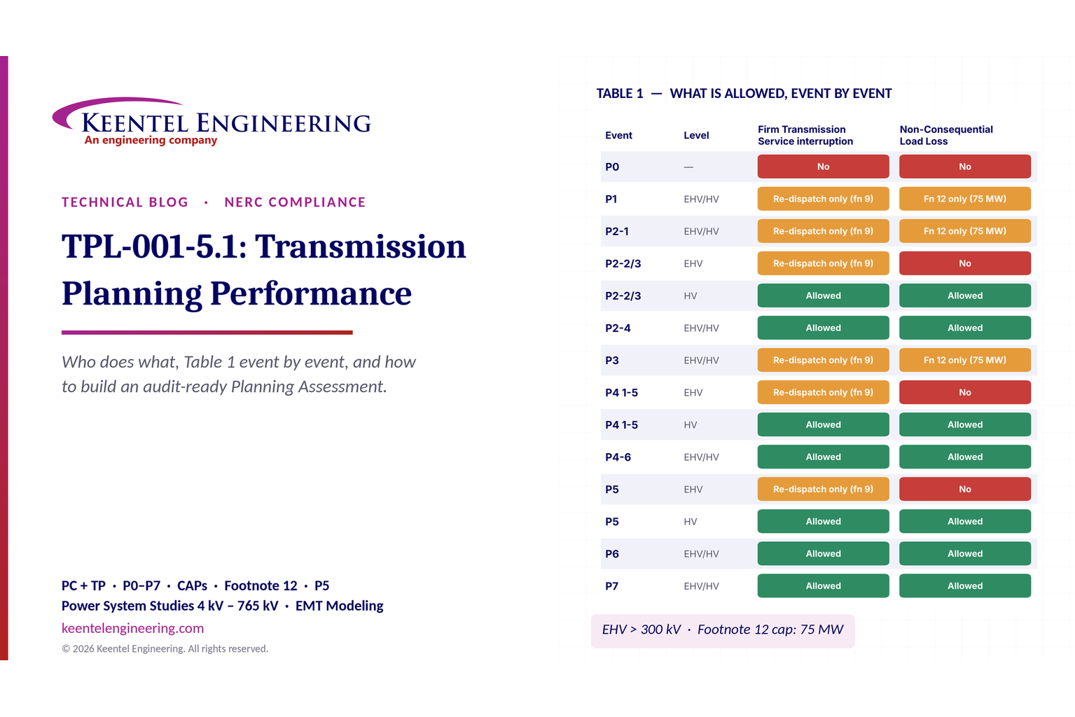
By SANDIP R PATEL
•
November 8, 2026
Explore NERC TPL-001-5.1 requirements, P0–P7 planning events, Table 1, corrective action plans and annual assessments with Keentel Engineering.
By SANDIP R PATEL
•
November 6, 2026
Compare radial vs. loop distribution systems in the US. Explore reliability, underground cables, protection, voltage drop and design with Keentel Engineering.