
A Coordinated Electric System Interconnection Review—the utility’s deep-dive on technical and cost impacts of your project.
Challenge: Frequent false tripping using conventional electromechanical relays
Solution: SEL-487E integration with multi-terminal differential protection and dynamic inrush restraint
Result: 90% reduction in false trips, saving over $250,000 in downtime
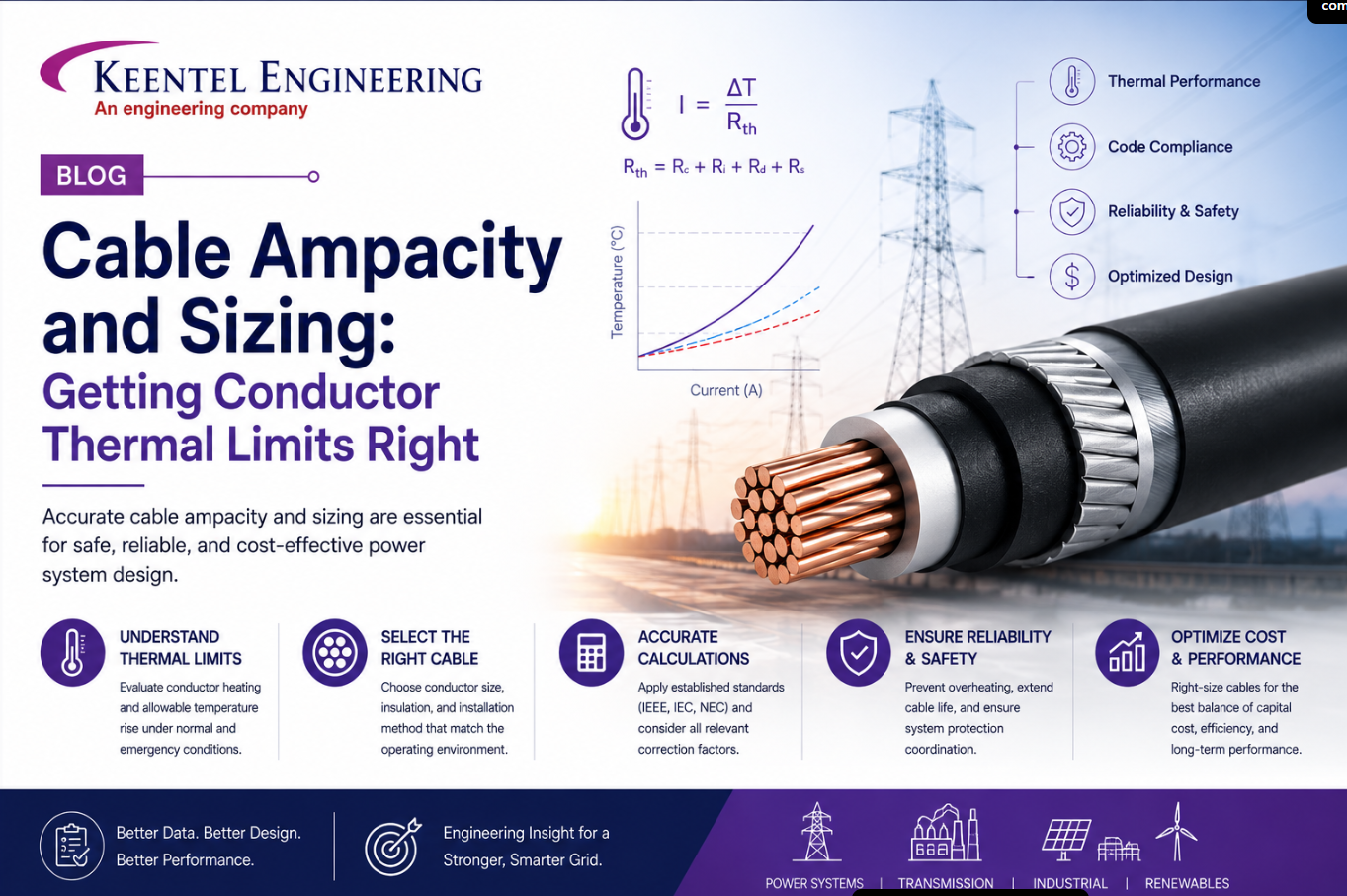
Cable Ampacity and Sizing: Getting Conductor Thermal Limits Right
Jun 8, 2026 | Blog
Cables are the part of a power system that engineers tend to take for granted right up until one of them runs too hot. They carry everything from lighting circuits to the feeders behind a substation or a hyperscale load, and they fail quietly: not with a bang, but with insulation that ages a little faster every time the conductor sits above its rated temperature. Get the size right and a cable will run reliably for decades. Get it wrong and you are trading service life for a few dollars of copper, or worse, courting a fault.
Ampacity is the discipline that prevents that trade from happening by accident. This article walks through what ampacity actually is, why a single number off a manufacturer's data sheet is almost never the right answer, the three methods engineers use to arrive at a defensible figure, and how the standards and modern study tools fit together in practice.
Ampacity is a thermal problem, not an electrical one
Ampacity — called current-carrying capacity in IEC practice — is the maximum continuous current a conductor can carry without exceeding its temperature rating. The word "temperature" is doing all the work in that sentence. When current flows through a conductor it dissipates power as heat at a rate of I²R watts, and that heat has to leave the cable by conduction and convection into whatever surrounds it. The conductor settles at whatever temperature balances heat generated against heat removed. Ampacity is simply the current at which that equilibrium lands exactly on the insulation's temperature limit.
This is why ampacity cannot be read off a table and trusted. The same cable that carries 530 A in open air may carry barely half that buried in a crowded duct bank, because the duct bank removes heat far more slowly. The conductor has not changed; its thermal environment has. Every factor that affects ampacity is ultimately a factor that affects how fast heat escapes:
- Cable construction — conductor material and size, and the insulation, sheath, armor, and bedding layers the heat must cross.
- Installation method — direct buried, in duct, in tray, in conduit, or in free air, each with a different thermal path.
- Ambient temperature — the baseline the conductor's heat rise stacks on top of.
- Grouping — neighboring loaded cables warm each other and slow each other's heat loss.
- External heat sources — an adjacent steam line or process pipe raises the local ambient.
- Soil thermal resistivity — for buried installations, how readily the surrounding earth conducts heat away.
- Harmonics — current at frequencies above the fundamental adds heating beyond what the RMS value alone suggests.
- Solar radiation and fire protection — sunlight loads exposed cable thermally; fire coatings and wraps insulate it and reduce ampacity.
The exact reference conditions matter because they define what "base ampacity" even means. A typical underground base ampacity is quoted at 20 °C ambient, a 90 °C conductor operating temperature, and a soil thermal resistivity of 90 °C·cm/W; above-ground base values use their own reference set. The base figure is a promise that holds only under those exact conditions — and real installations almost never match them.
Base ampacity, derating, and the conductor-temperature lever
Because the reference conditions rarely reflect reality, the base value gets adjusted. There are two ways to do this: a full thermal analysis, or the application of correction (derating) factors. The factor-based approach is the everyday workhorse — you take the base ampacity and multiply it by every applicable derating factor to get the derated ampacity, which is the number you actually design against.
Two derating factors apply to essentially every installation: ambient temperature and allowable conductor temperature. The rest depend on where and how the cable runs. Underground installations add soil thermal resistivity, grouping, and mutual heating from neighboring circuits. Above-ground installations add grouping within trays, fire protection, and solar exposure.
The conductor-temperature factor deserves special attention because engineers underuse it as a design lever. A 90 °C-rated cable does not have to be operated at 90 °C. If you deliberately limit its operating temperature to 75 °C — to extend insulation life, or to leave thermal headroom for future load — the derated ampacity can drop by nearly half. That is not a penalty; it is a knob. The same physics that punishes a hot, crowded duct bank rewards a conservatively operated conductor with a longer service life.
Three methods to determine ampacity
Engineers reach a defensible ampacity figure by one of three routes. They are not competitors so much as tools for different jobs.
1. Full thermal analysis.
This computes the cable's thermal behavior directly rather than relying on tabulated factors. The two established methods are Neher-McGrath — the analytical method that underpins most North American underground practice — and the calculation procedure in IEC 60287; finite element methods handle the genuinely awkward geometries. Thermal analysis applies to underground duct banks and direct-buried installations, and it is the most comprehensive option because it can account for arbitrary duct-bank shapes, real spacing, and explicit external heat sources. It is also the most computation-intensive, which is why it is reserved for cases where squeezing real margin out of a congested underground run justifies the effort.
2. Manufacturer base ampacity with correction factors.
Here the manufacturer supplies a base ampacity for a defined installation, and you apply derating factors for the actual ambient, grouping, soil, and so on. This is the model behind the IEEE 399 / Brown Book approach.
3. Standard ampacity tables with rating factors.
The standard itself provides both the base ampacities and the rating factors in tabular form — you look up the base value and the applicable factors and combine them. NEC and IEC 60364 work this way.
One method resists tidy classification. ICEA P-54-440, used for above-ground cable trays, looks like a table method but behaves like a semi-thermal calculation: there is no base ampacity to derate from. Instead the method computes the tray ampacity directly from the tray geometry — height, width, and percent fill. A 750 kcmil cable in a 6-inch by 18-inch tray at 30% fill, for instance, resolves to a single calculated figure with no manufacturer base value in sight. Fire protection then derates
that result: a one-inch fire coating might pull the same cable down by roughly 14%, with further reductions for wraps and for fire stops at wall penetrations.
How the standards divide up the work
It helps to know which standard owns which installation, because picking the wrong one produces a perfectly precise answer to the wrong question.
On the ANSI / 60 Hz side, IEEE 399 (the Brown Book, now carried within the IEEE 3002 series) covers direct-buried and duct-bank installations and is the usual choice for industrial, mostly medium-voltage work. Its tables were built from thousands of underground cable studies and assume a uniform duct bank at 7.5-inch center-to-center spacing with every conduit filled by the same cable size, sizing so that the hottest location — the lowest, most thermally trapped point in the bank — sits at 90 °C. A 3×5 bank under that assumption might yield 192 A per conductor across all fifteen conduits. ICEA P-54-440 owns above-ground trays and leans commercial. NEC Article 310 provides base ampacities for above-ground trays, conduits, and air drops, with tray adjustments for top covers and maintained spacing.
On the international side, IEC 60364 covers low-voltage installations (≤1 kV AC / ≤1.5 kV DC) and supports the widest range of installation methods of any standard — conduit in air, underground duct, trenches, voids through buildings, wire mesh, and more. BS 7671 tracks IEC closely, with similar methodology, different tables, and a few more correction factors; results sometimes coincide and sometimes don't. IEC 60502 handles medium voltage, with IEC 60092 (marine/offshore), the French NFC 15-100 and 13-200, AS/NZS 3008, and the German VDE 0298-4 rounding out regional coverage.
A subtle but important difference among these is where the base ampacity lives. For IEEE 399 it comes from the cable library / manufacturer data and cannot be edited. For NEC it comes from the Article 310 tables. For IEC 60364 and BS 7671 it comes from the standard's own tables rather than the library, and some parameters — like the 90 °C conductor temperature IEC fixes, or the 85 °C a particular BS 7671 cable enforces — are locked by the standard and not yours to change.
From ampacity to a sized conductor
Ampacity tells you how much current a cable can carry. Sizing asks the inverse: given the load, what conductor do I need? In practice the two run together, and sizing is governed by constraints, of which loading and voltage drop are the two you cannot skip.
Loading can be defined three ways. The operating current pulls the actual amps from a load-flow study (or from real-time field measurements), which is the most representative basis and the usual default. The full-load-amps-of-element option senses the rating of a connected device — useful when a cable feeds a transformer or motor and you want to size to the equipment rather than the present load; sizing to a 600 A switchgear, for instance. Or you can simply enter a user-defined value when an internal derating table or a known future load governs.
Voltage drop becomes the binding constraint on long runs. NEC practice targets 3% through a branch, and a good study tool will return the maximum length at which a given size still meets that limit — past roughly 1,500 feet on a moderate feeder the drop, not the heat, often decides the size. Short-circuit withstand adds a third constraint: the conductor must survive the fault energy (I²t) set by the available fault current and the clearing time of its upstream protective device, both of which come straight from the short-circuit study and the device's time-current behavior. Overload, zero-sequence, triple-harmonic, and minimum-conductors-per-phase constraints layer on as the application demands.
The result is an optimal size — and often a one-size-smaller alternative worth a hard look. Sizing convention assumes 100% loading (with a 1.25 multiplier on the largest motor when sizing an MCC), but if the load realistically never exceeds 70–80%, the smaller conductor may carry the duty at real savings. The discipline is to make that call explicitly, with the headroom numbers in front of you, rather than defaulting either way.
Where the workflow comes together
The reason all of this is worth doing inside an integrated study environment rather than a spreadsheet is that ampacity does not live alone. A load-flow run will flag any cable loaded past 100% of its derated limit as an alert and paint it red on the one-line — the digital equivalent of an operator's overload alarm. Pushing those load-flow amps into the cable editor (via the study-case "cable load amps" update) makes the sizing calculation reflect the real connected load, not an assumption. Resize the conductor, rerun the load flow, and the alert clears. A cable manager then rolls every cable in the project into one view — base, operating, and derated ampacity, installation type, constraints, and violation flags side by side — so the analysis scales from one feeder to an entire facility, with reports exportable to PDF or spreadsheet at the end.
That integration is the real point. Ampacity, voltage drop, short-circuit withstand, and load flow are facets of one question — will this conductor do its job safely for its design life? — and answering it well means treating them as one study, not four.
Case Studies
All case studies are anonymized. Client names, locations, and project identifiers have been removed.
Case Study 1 — Resizing an overloaded medium-voltage duct-bank feeder
Background.
A large industrial facility commissioned a power-system study after a feeder serving a downstream switchgear lineup began tripping intermittently under full production load. The feeder ran underground through a multi-row duct bank shared with several other circuits.
Challenge.
A load-flow analysis immediately flagged the feeder as critically overloaded. Its derated ampacity worked out to roughly 89 A, while the actual operating current under full load was close to 288 A — an overload exceeding 300% of the conductor's real limit. The original design had used the cable's base ampacity without accounting for the duct bank's grouping effect. With the circuit modeled as part of a populated bank under the IEEE 399 method, the grouping and ambient corrections collapsed the usable ampacity to a fraction of the base figure.
Approach.
We modeled the duct bank with its true row-and-column configuration so the derated ampacity reflected the real thermal environment, then drove the sizing calculation from the load-flow operating current rather than a nameplate assumption. Loading and a 3% voltage-drop limit were set as the binding constraints. The calculation returned an optimal solution of two conductors per phase in parallel, sized so that the combined ampacity (~298 A) comfortably exceeded the 288 A load while holding voltage drop near 0.1%.
Outcome.
With the parallel arrangement in place, a re-run of the load flow cleared the overload alert entirely. The exercise also produced a documented derating basis for the rest of the duct bank, so the same grouping error would not recur on adjacent circuits. The root cause — designing to base rather than derated ampacity — was corrected as a standing practice, not just for the one feeder.
Case Study 2 — Fire-protection derating in a commercial cable-tray distribution system
Background.
A commercial campus with a dense above-ground cable-tray distribution network required an ampacity review after a fire-stopping retrofit was added at every wall and floor penetration. The original tray ampacities had been established before the fire protection was specified.
Challenge.
The tray cables had been sized using a semi-thermal tray calculation (ICEA P-54-440), with ampacity derived directly from tray geometry and fill. The retrofit added fire coatings along sections of tray and fire wraps and stops at penetrations — all of which act as thermal insulation. None of this had been carried into the original ampacity basis, leaving several heavily loaded runs at risk of operating above their true derated limit once the fire protection was installed.
Approach.
We recomputed the tray ampacities with the fire protection included as a derating factor rather than an afterthought. On the most affected runs, the fire coating alone reduced the calculated ampacity by roughly 14%, with further reductions at the wrapped penetrations. Where the derated figure no longer covered the connected load, we evaluated two remedies: increasing conductor size on the constrained runs, and reducing tray fill to restore heat dissipation. The percent-fill sensitivity of the semi-thermal method made the fill-reduction option quantifiable rather than a guess.
Outcome.
A combination of selective upsizing and reduced fill on the worst runs brought every circuit back within its derated limit, with the fire protection fully accounted for. The review established that fire-protection derating would be incorporated at design time on all future tray work, closing a gap that the retrofit had exposed.
Case Study 3 — Installation-method selection and a thermal cross-check on an international low-voltage project
Background.
A facility built to international (IEC) practice required low-voltage cable sizing across a mix of installation conditions — cable trays, conduit in air, and a congested underground duct section running near a process heat source.
Challenge.
The project spanned installation methods that no single table cleanly covered, and the client's specification fixed the conductor temperature by standard, removing it as a design variable. The underground section was the concern: several circuits shared a duct bank close to a heated process line, and the table-based grouping factors alone could not confirm whether the proximity heat source would push conductors past their limit.
Approach.
For the above-ground and in-air runs we applied IEC 60364, using its broad set of installation types to match each run precisely — including choosing perforated over unperforated trays where airflow mattered, which measurably raised the achievable ampacity. We cross-referenced selected runs against BS 7671, whose closely related but more numerous correction factors gave a useful second opinion. For the congested underground section we set the table methods aside and ran a full thermal analysis (Neher-McGrath / IEC 60287) with the process heat source modeled explicitly. The thermal model showed that, with the heat source active, the lowest conductors in the bank would exceed the standard's temperature limit at the table-based ampacity.
Outcome.
The thermal analysis justified increasing spacing in the duct bank and upsizing the two most-affected circuits — a change the table method would not have identified, because it could not represent the external heat source. The above-ground runs were sized efficiently against the correct installation types, and the underground section gained a defensible margin against a heat source that a tables-only approach would have missed. The project illustrated the right division of labor: table methods for the routine runs, full thermal analysis where an unusual thermal environment demanded it.
Frequently Asked Questions
Which standard applies to my installation?
Roughly: IEEE 399 / Brown Book for industrial underground duct banks and direct-buried runs (mostly MV); ICEA P-54-440 for above-ground cable trays (commercial); NEC Article 310 for above-ground trays, conduits, and air drops in North America. Internationally, IEC 60364 and BS 7671 for low-voltage work, IEC 60502 for medium voltage, with regional standards (NFC, AS/NZS, VDE, IEC 60092) as jurisdiction requires.
What is the difference between base ampacity and derated ampacity?
Base ampacity is the current a cable can carry under a specific set of reference conditions (for underground, typically 20 °C ambient, 90 °C conductor temperature, and 90 °C·cm/W soil thermal resistivity). Derated ampacity is that base value adjusted by correction factors for the cable's actual installation — ambient, grouping, soil, fire protection, and so on. You design against the derated value, because that is the real limit.
Why can't I just use the manufacturer's published ampacity?
Because the published figure assumes the manufacturer's reference installation, which your installation almost certainly doesn't match. A cable rated for a single circuit in open air behaves very differently buried in a multi-row duct bank surrounded by other loaded conductors. The published number is a starting point to be derated, not an answer.
What are the three methods for determining ampacity?
Full thermal analysis (Neher-McGrath, IEC 60287, or finite element), which computes thermal behavior directly; manufacturer base ampacity adjusted by correction factors; and standard ampacity tables combined with the standard's rating factors. Thermal analysis is the most rigorous and the most computation-heavy; the factor and table methods are faster and adequate for most everyday work.
When should I use full thermal analysis instead of the table or factor methods?
For underground duct banks and direct-buried runs where you need to extract real margin, account for an unusual duct-bank geometry, model explicit external heat sources, or justify a tighter design than the conservative table assumptions allow. For routine above-ground tray and conduit work, the standard-based methods are normally sufficient.
Why is ICEA P-54-440 described as "semi-thermal"?
Because, unlike a true table method, it has no base ampacity to derate. It calculates the tray ampacity directly from tray geometry — height, width, and percent fill. There is no manufacturer base value in the chain. It looks tabular in the published standard but behaves like a calculation.
How does grouping reduce ampacity?
Loaded cables in proximity heat one another and slow each other's ability to shed heat. In a duct bank, adding rows or columns of conduits lowers the derated ampacity of every cable, because the bank as a whole holds heat longer. The Brown Book captures this by assuming a uniform, fully populated bank and sizing so the hottest, most thermally trapped location stays at the temperature limit.
Does limiting the operating temperature below the cable's rating reduce its ampacity?
Yes, substantially. Operating a 90 °C-rated cable at a 75 °C limit can cut the derated ampacity by close to half. This is sometimes done deliberately to extend insulation life or reserve thermal headroom — it is a legitimate design choice, not just a constraint.
Do fire coatings and wraps affect ampacity?
Yes. Fire coatings, wraps, and stops are thermal insulation, so they reduce a cable's ability to shed heat and therefore lower its ampacity. A one-inch fire coating can reduce a tray cable's rating by roughly 14%, with additional reductions for wraps and for fire stops at wall penetrations. These must be accounted for, not added after sizing.
What's the difference between operating, full-load-amps-of-element, and user-defined loading for sizing?
Operating current uses the actual amps from a load-flow study (or field measurements) — the most representative basis and usual default. Full-load-amps-of-element sizes to a connected device's rating (a transformer or switchgear), useful when you want to match the equipment rather than present load. User-defined lets you enter a specific value when an internal table or known future load governs.
When does voltage drop, rather than heat, decide the cable size?
On long runs. Ampacity usually governs short, heavily loaded feeders, but as length grows, voltage drop takes over — NEC practice targets 3% through a branch. A good study tool reports the maximum length at which a given size still meets that limit, which makes the crossover obvious.
Should I ever choose one size smaller than the calculated optimal?
Sometimes. The optimal size assumes 100% loading. If the load realistically peaks at 70–80%, the next size down may carry the duty with real material savings. It can also suit feeders only briefly overloaded during maintenance or bus transfers. Make the call explicitly, with the headroom figures in view — and note that MCC sizing conventionally adds a 1.25 multiplier on the largest motor, which usually argues against undersizing.
How does ampacity analysis connect to load flow and short-circuit studies?
Tightly. Load flow supplies the operating current and flags any cable past its derated limit; short-circuit results supply the fault current and clearing time that set the short-circuit sizing constraint. Treating ampacity, voltage drop, short-circuit withstand, and load flow as one integrated study — rather than four separate exercises — is what keeps the answers consistent.

About the Author:
Sonny Patel P.E. EC
IEEE Senior Member
In 1995, Sandip (Sonny) R. Patel earned his Electrical Engineering degree from the University of Illinois, specializing in Electrical Engineering . But degrees don’t build legacies—action does. For three decades, he’s been shaping the future of engineering, not just as a licensed Professional Engineer across multiple states (Florida, California, New York, West Virginia, and Minnesota), but as a doer. A builder. A leader. Not just an engineer. A Licensed Electrical Contractor in Florida with an Unlimited EC license. Not just an executive. The founder and CEO of KEENTEL LLC—where expertise meets execution. Three decades. Multiple states. Endless impact.
Services

Let's Discuss Your Project
Let's book a call to discuss your electrical engineering project that we can help you with.
About the Author:
Sonny Patel P.E. EC
IEEE Senior Member
In 1995, Sandip (Sonny) R. Patel earned his Electrical Engineering degree from the University of Illinois, specializing in Electrical Engineering . But degrees don’t build legacies—action does. For three decades, he’s been shaping the future of engineering, not just as a licensed Professional Engineer across multiple states (Florida, California, New York, West Virginia, and Minnesota), but as a doer. A builder. A leader. Not just an engineer. A Licensed Electrical Contractor in Florida with an Unlimited EC license. Not just an executive. The founder and CEO of KEENTEL LLC—where expertise meets execution. Three decades. Multiple states. Endless impact.
Leave a Comment
Thank you for contacting us.
We will get back to you as soon as possible.
We will get back to you as soon as possible.
Oops, there was an error sending your message.
Please try again later.
Please try again later.
Related Posts
By SANDIP R PATEL
•
July 23, 2026
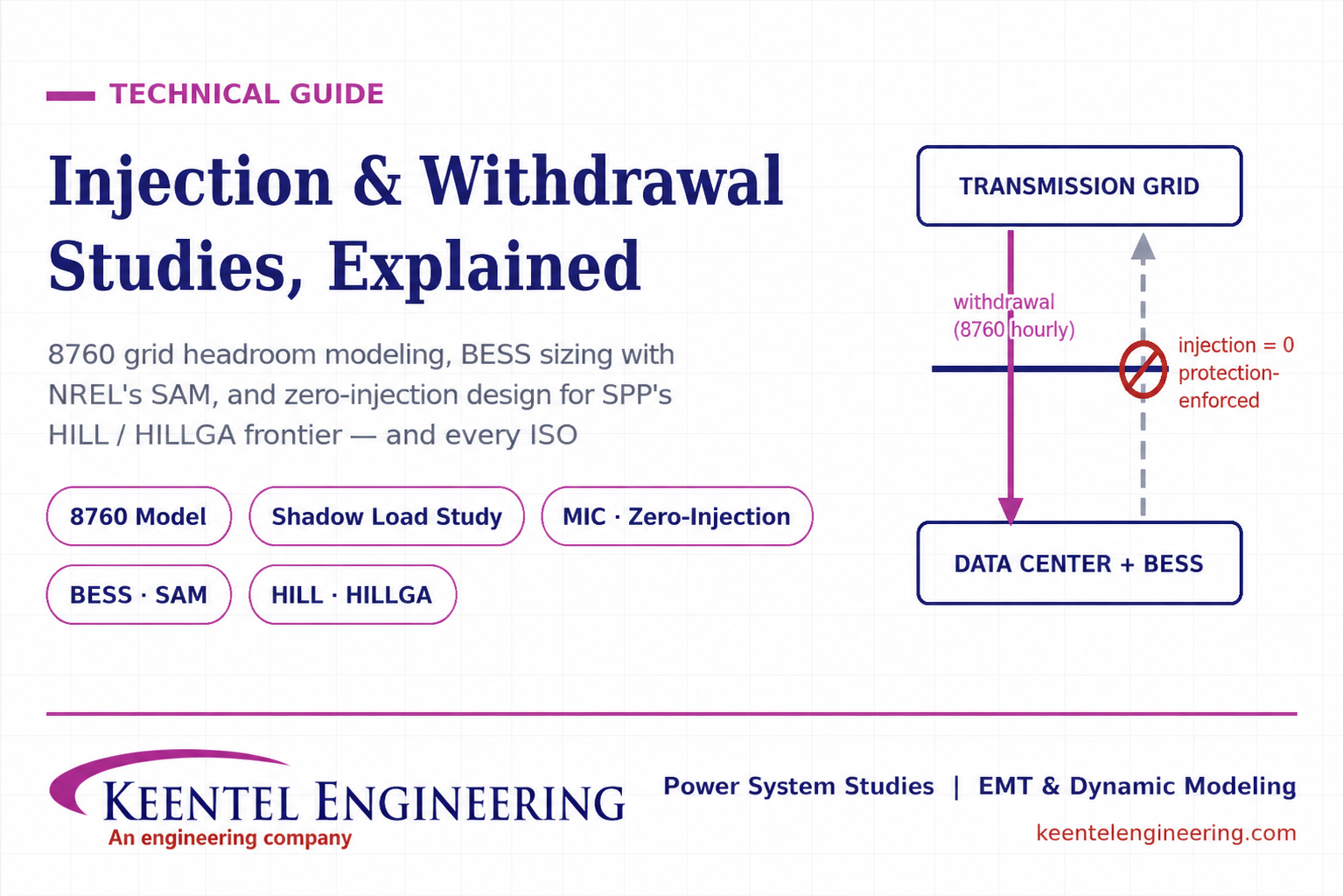
Learn how injection and withdrawal studies, 8760 headroom modeling, zero-injection engineering, and SPP HILLGA improve large load grid interconnections
By SANDIP R PATEL
•
July 21, 2026
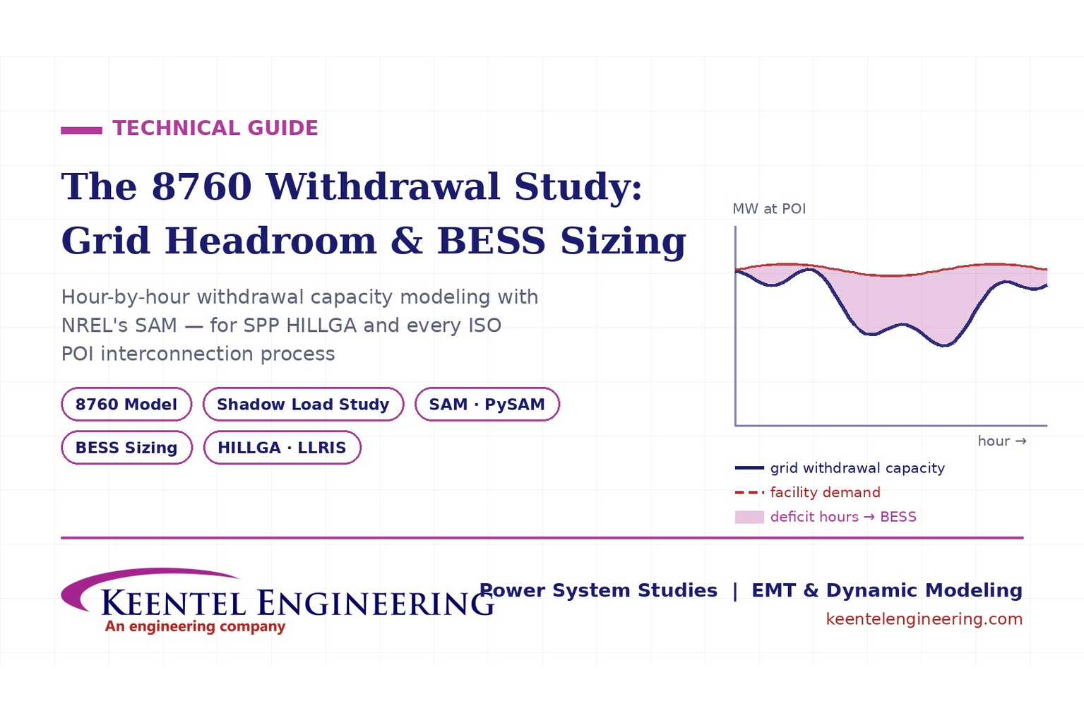
Learn how an 8760 withdrawal study models hourly grid headroom and uses SAM-based BESS sizing for large-load interconnection projects.
By SANDIP R PATEL
•
July 21, 2026
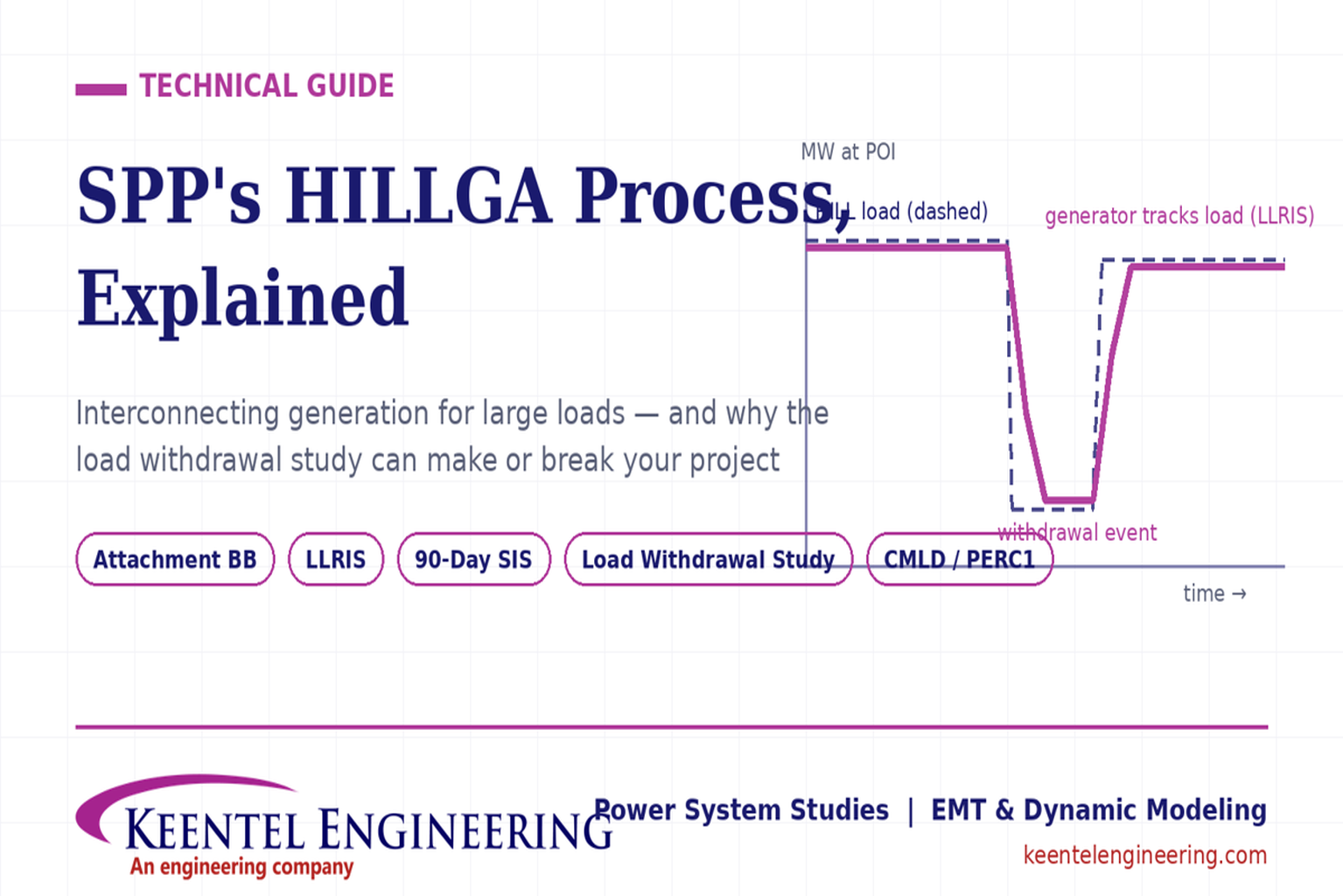
Learn how the SPP HILLGA process supports data center generation interconnection and why an 8760 withdrawal study can determine project success.
By SANDIP R PATEL
•
July 19, 2026
Learn electrical protection and relay coordination for hyperscale data centers with IEEE standards, short-circuit studies, arc-flash analysis, and MV protection.

By SANDIP R PATEL
•
July 18, 2026
Explore Battery Energy Storage System components, including cells, PCS, BMS, EMS, cooling, fire protection, sizing, safety, and grid codes.

By SANDIP R PATEL
•
July 18, 2026
Explore how grid-forming inverters support BESS, synthetic inertia, grid-code compliance, plant sizing, testing, and project revenue.
By SANDIP R PATEL
•
July 18, 2026
Learn how SEL RTAC protection monitoring supports NERC PRC-005 compliance, predictive maintenance alarms, automated reporting, and relay verification.

By SANDIP R PATEL
•
July 17, 2026
Explore utility-scale BESS design from the 10% package to IFC, NFPA 855 compliance, PSS®E/PSCAD models, and ERCOT interconnection.
By SANDIP R PATEL
•
July 17, 2026
Substation design guide, electrical substation design, substation equipment sizing, IEEE 80 grounding design, IEEE 998 lightning shielding, bus configuration design