A Coordinated Electric System Interconnection Review—the utility’s deep-dive on technical and cost impacts of your project.
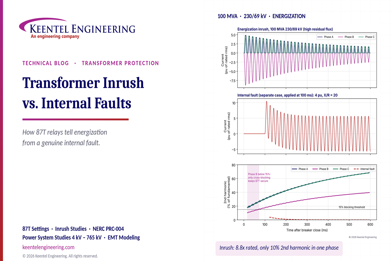
Challenge: Frequent false tripping using conventional electromechanical relays
Solution: SEL-487E integration with multi-terminal differential protection and dynamic inrush restraint
Result: 90% reduction in false trips, saving over $250,000 in downtime
The three operating regions you have to design to
| Device | Output vs voltage | Response | Best suited to | Main limitations |
|---|---|---|---|---|
| Mechanically switched capacitor or reactor | Proportional to voltage squared | Seconds; discrete steps; limited switching operations per day | Steady-state reactive supply, voltage profile, loss reduction | No dynamic capability; step voltage change on switching; capability collapses when most needed |
| Static var compensator | Capacitive branches proportional to voltage squared | A few cycles; continuously controllable | Continuous control where cost matters and deep voltage support is not the driver | Square-law capability loss; harmonic filters are part of the plant and interact with the network |
| STATCOM | Approximately proportional to voltage — constant current capability | One to two cycles closed loop; converter response faster still | Voltage stability margin, weak interconnections, fast disturbance recovery, flicker and unbalance compensation | Higher capital cost; converter losses; adds a converter and its control dynamics to the network |
| Synchronous condenser | Governed by machine capability and excitation | Excitation response in the hundreds of milliseconds; inherent inertial response instantaneous | System strength and inertia, short-circuit contribution, black start support | Rotating plant with maintenance and losses; slower controlled response than a converter |
| STATCOM with energy storage | Reactive as a STATCOM, plus real power within the storage rating | As STATCOM for reactive; real power limited by storage | Where a real power deficiency is part of the problem | Cost and complexity of the storage; different failure and maintenance profile |
| Service area | What we do for SST campuses | Typical deliverables |
|---|---|---|
| Grid interconnection | Site screening, large-load applications, independent studies, utility and RTO coordination in ERCOT, NYISO, PJM and other markets | Screening reports, application data packages, load flow, contingency and stability studies, study review memos |
| EMT modeling | Model requirements, vendor model review, campus aggregation, ride-through, weak-grid, control interaction and load-oscillation studies | EMT model specifications, model acceptance reports, PSCAD study reports, SCR screening |
| MV/MVDC system studies | AC and DC short-circuit, DC protection philosophy, AC protection, arc flash, grounding, insulation coordination | Study reports, protection philosophy documents, settings files, arc flash labels, interface control documents |
| Power quality | Emission requirements, frequency scans, IEEE 519-2022 compliance, filter sizing, flicker assessment | Harmonic study reports, filter specifications, monitoring plans |
| Substation and transmission design | HV/EHV substations, MV collectors, transmission lines, utility interface protection | Physical and electrical drawing packages, specifications, bills of material, protection and control design |
| NERC compliance | Registration and applicability, ride-through requirements, model validation, monitoring, compliance programs | Applicability assessments, compliance programs, evidence packages, model validation reports |
| Owner's engineer and QA/QC | SST, storage and substation specifications, design reviews, FAT and SAT plans and witnessing, multi-unit QA | Specifications, review comments, test plans, witness reports, due diligence reports |
| Onsite generation and BESS | Role definition and sizing, DC bus control architecture, fire and code compliance coordination, performance testing | Sizing studies, control architecture documents, specifications, test procedures |
Storage and generation
| Term | Meaning |
|---|---|
| AFE | Active front end. The actively switched AC/DC stage of an SST that connects to the MV grid and sets its grid behavior. |
| Aggregated model | A model in which many converters are represented by a smaller number of equivalent converters to make campus-scale simulation practical. |
| Arc flash | The release of energy from an electric arc fault, assessed as incident energy at a working distance to set PPE and safe work practices. |
| BESS | Battery energy storage system. |
| Blocking | Turning off all converter switches so the converter stops feeding current, used to limit DC faults. |
| Composite load model | A positive-sequence load model that combines several load types, such as motors, electronics and static loads. |
| DAB | Dual active bridge. An isolated DC/DC converter topology with active bridges on both sides of a high-frequency transformer. |
| DC-link | The internal DC capacitor bank between converter stages. |
| EMT | Electromagnetic transient simulation. Time-domain simulation with microsecond time steps, used to study fast converter and network behavior. |
| FAT | Factory acceptance test. |
| Grid-forming | A converter control mode that sets its own voltage and frequency reference rather than following the grid's, providing support to weak grids. |
| HIL | Hardware-in-the-loop testing, in which a real controller is tested against a real-time simulation. |
| IBR | Inverter-based resource. Generation or storage connected to the grid through power electronics. |
| Insulation coordination | Matching the insulation strength of equipment to the voltage stresses the system produces, with surge protection where needed. |
| ISC/IL | The ratio of available short-circuit current to maximum demand load current at the point of common coupling, used to set IEEE 519 limits. |
| ISOP | Input-series, output-parallel. A modular converter arrangement that shares a high input voltage across cells in series and combines their outputs in parallel. |
| Large load | A load large enough to affect transmission system reliability. Definitions vary, for example 75 MW and above under Texas SB 6, or loads above 20 MW in the federal rulemaking proposal. |
| LVDC | Low-voltage DC, such as 800 VDC or ±400 VDC rack distribution. |
| MFT | Medium-frequency transformer. The compact isolation transformer inside an SST, operating at kilohertz frequencies. |
| MMC | Modular multilevel converter. A converter built from many submodules with their own capacitors, producing a stepped multilevel waveform. |
| MVDC | Medium-voltage DC distribution, roughly 1 kV to 35 kV DC in common usage. |
| OE | Owner's engineer. An independent engineer representing the owner's technical interests. |
| PCC / POI | Point of common coupling / point of interconnection, where the campus connects to the utility system and where compliance is usually assessed. |
| PLL | Phase-locked loop. The control element that tracks grid voltage phase and frequency. |
| Positive-sequence model | A fundamental-frequency, balanced dynamic model used in PSS®E, PSLF and similar tools. |
| Ride-through | The ability to stay connected and keep operating during and after a grid disturbance within defined limits. |
| SAT | Site acceptance test. |
| SCR | Short-circuit ratio. Available short-circuit power divided by converter rating, a measure of grid strength. |
| SiC | Silicon carbide, a wide-bandgap semiconductor material that allows higher voltage, higher frequency switching. |
| SST | Solid-state transformer. A power electronic converter with a high-frequency isolation stage that replaces a 60 Hz transformer and rectifier chain. |
| Supraharmonics | Emissions in the 2 kHz to 150 kHz range, above the range covered by most harmonic limits. |
| TDD | Total demand distortion. Harmonic current distortion relative to maximum demand current, used in IEEE 519. |
| WSCR | Weighted short-circuit ratio. An SCR screen that accounts for several inverter-based plants sharing a network area. |
Links were current at publication (November 2026). Large-load rules, NERC actions and standards editions are changing quickly, so confirm current versions before relying on them.
Large-load reliability and NERC
- NERC Publishes Incident Review and Guidance on Voltage-Sensitive Large Load Integration, NERC
- Reliability Insights: Large Computational Load Risks Due to Voltage Sensitivity, NERC, September 2026
- NERC Seeks to Address Reliability Impacts from Large Load Integration, NERC presentation to FERC, April 2025
- NERC issues Level 3 Alert to address immediate risks data center loads pose to the grid, Renewable Energy World, May 2026
- NERC Voltage-Sensitive Loads, Keentel Engineering
Federal and state large-load rules
- FERC Docket RM26-4, Interconnection of Large Loads, FERC
- FERC Establishes Proceeding to Consider DOE Directive on Large Load Transmission Interconnection Rulemaking, McGuireWoods, October 2025
- Texas Senate Bill 6 Ushers in Major Overhaul of Large Load Interconnection and Grid Access Rules, Bracewell, July 2025
- Public Utility Commission of Texas Issues Proposed Rules for Large Load Interconnections, Foley & Lardner, March 2026
Solid-state transformers and DC data center power
- Solid State Transformer project, Open Compute Project
- Novel Solid-State Transformer Supports 800-V DC Power in AI Data Centers, Electronic Design
- How SSTs are Reshaping Data Center Infrastructure, Microchip Technology
Standards referenced (consult the publisher for the current edition)
Step 5 — options. Replacing or retrofitting the drives with active-front-end or 18-pulse units at about 5% THDi gives a TDD of about 1.5%. An active harmonic filter sized for the 5th and 7th could achieve a similar result at the facility level. A passive 5th-harmonic tuned filter would also work but must be checked for resonance with the utility system and with any future capacitors.
What this means for you.
The same drives can be compliant on a strong system and non-compliant on a weak one. Ask your utility for the maximum short-circuit current at the PCC early in design. If the ratio is below 50, plan for low-harmonic drives or filtering from the start; it is much cheaper than retrofitting.
9. Inverter-based resources: solar, storage and wind
Solar PV, battery energy storage and full-converter wind turbines use pulse-width-modulated inverters with output filters. They are generally low-distortion sources. IEEE Std 1547-2018 (distribution-connected resources) and IEEE Std 2800-2022 (transmission-connected resources) limit their current distortion — total rated-current distortion (TRD) of 5% with individual limits by order, measured against rated current rather than present output. In practice, quality inverters measure 1–3% at rated output.
Three cautions apply:
- Percentages rise at low output. At 10% of rated output a 2% distortion (of rated current) looks like 20% THD. Limits referenced to rated current, like TDD, avoid this trap.
- Inverters change the system's impedance. Plant collector cables, inverter output filters and capacitor banks add capacitance. They can create resonances near the 5th to 13th harmonics on the 34.5 kV collector or at a 138 kV, 230 kV or 345 kV point of interconnection, amplifying background distortion that the plant did not create.
- Background distortion matters. Inverters can absorb or amplify existing voltage distortion depending on their control design. Utilities increasingly require harmonic impedance studies for new plants, sometimes using electromagnetic transient (EMT) simulation.
Keentel's articles on harmonic resonance and on
weak-grid inverter stability cover these interactions in depth.
10. Data centers and other electronic facilities
Data centers are a special case because almost all their load is electronic. Points to check:
- UPS rectifiers. Double-conversion UPS units with IGBT rectifiers typically draw less than 5% THDi at rated load, rising at low load. Older six-pulse or 12-pulse thyristor UPS rectifiers may need input filters.
- Server and network power supplies. Modern units with active power factor correction have low 3rd harmonic. Legacy equipment does not. Measure a representative panel rather than assuming.
- 208Y/120 V and 415Y/240 V distribution. Check neutral current and transformer K-factor as in Sections 4 and 7.
- Generator operation. Test UPS and generator compatibility at the actual load level. Generator THDv can be three to four times the utility THDv for the same load.
- Cooling plant. Chiller, pump, fan and cooling distribution unit drives often contribute more low-order harmonics than the IT load. Specify low-harmonic drives where the facility is large relative to the utility source.
- Large-load interconnection. Utilities and grid operators now treat large data centers as high-impact loads. Harmonic studies and power quality monitoring are increasingly part of interconnection requirements, alongside ride-through and dynamic studies.
11. How a harmonic study is done
A harmonic study answers four questions: How much harmonic current will the facility inject? What voltage distortion will it cause? Will any resonance amplify it? What is the cheapest reliable fix? Keentel's typical workflow:
- Gather data. Single-line diagram; utility short-circuit data (maximum and minimum) at the PCC; utility background distortion if known; transformer impedances; cable lengths; capacitor banks and filters; drive, UPS and inverter data sheets with harmonic spectra.
- Measure existing conditions. For existing facilities, install class-compliant power quality meters at the PCC and key buses for at least one week, capturing 10-minute and 3-second data up to the 50th harmonic.
- Build the model. Represent sources as harmonic current injections and the network as frequency-dependent impedances, including transformer phase shifts that can cancel 5th and 7th harmonics between delta-delta and delta-wye units.
- Run a frequency scan. Plot driving-point impedance versus frequency at each important bus to find resonances, for all credible system configurations (tie breakers open/closed, capacitor steps in/out, generator versus utility).
- Run harmonic load flow. Calculate harmonic currents and voltages and compare them with IEEE 519 at the PCC and with equipment limits (IEEE 18 for capacitors, C57.110 for transformers) inside the facility.
- Design mitigation. Compare options for performance, cost, losses, footprint and future flexibility.
- Verify. Measure again after installation and document compliance with the statistical criteria.
12. Fixing harmonics: options compared
Closingthe Planning Gaps: How Transmission Improves Resource Adequacy in US Power Systems
November 06, 2026 | Blog
Part A — Resource Adequacy and Transmission Planning at a Glance
Every US utility, regional transmission organization (RTO) and state commission asks the same two questions about the future grid. Will there be enough generation, storage and demand response to serve load through the hottest summer afternoon and the coldest winter morning? And will the transmission network be able to deliver that supply where it is needed, reliably and at reasonable cost?
In most of the country those questions are answered by three separate processes, run by different organizations, on different schedules, with different models and different data:
- Resource adequacy (RA) assessments, run by balancing authorities, RTOs or utilities, estimate the probability of running short of supply and set the planning reserve margin (PRM) and resource accreditation rules.
- Resource planning — integrated resource plans (IRPs) at vertically integrated utilities and state agencies, and capacity expansion studies at RTOs — chooses the future generation and storage portfolio.
- Transmission planning, run by transmission owners (TOs) and regional planning entities, tests the future network against NERC reliability standards and, increasingly, economic and multi-value criteria.
Each process uses the outputs of the others, but usually from the previous cycle. Transmission topology and import limits enter the RA study as fixed assumptions. The future generation portfolio enters the transmission study as a fixed input. Nobody asks, inside one integrated model, whether a new 765 kV line or HVDC tie could replace a gigawatt of local peaking capacity at lower total cost.
Keentel Engineering calls these handoffs the planning gaps. This guide explains where they come from, why they raise costs for customers, how transmission actually delivers resource adequacy value, how to quantify that value with standard probabilistic methods, and what has changed with FERC Order No. 1920.
Keentel's companion article on cluster interconnection studies covers how individual generators connect to the grid under FERC Order No. 2023. This article looks one level up: how the system decides how much generation it needs and how much transmission should carry it.
The planning chain in one table
| Process | Who runs it | Typical horizon | Main model | Key outputs | How it treats the other processes |
|---|---|---|---|---|---|
| Resource adequacy assessment | Balancing authority, RTO, utility; NERC for interconnection-wide assessments | 1–10 years, often a single study year | Probabilistic (Monte Carlo or convolution) loss-of-load model, often one zone or a few zones | LOLE, LOLH, EUE; PRM; ELCC and accreditation values; import limits used for capacity | Transmission enters as fixed import or transfer limits, frequently from the prior planning cycle |
| Resource planning (IRP, capacity expansion) | States, utilities, RTOs | 15–25 years | Least-cost capacity expansion; zonal "pipe-and-bubble" transmission | Future generation and storage portfolio, retirements, costs | Must meet the PRM from the RA study; transmission is fixed or crudely represented |
| Transmission reliability planning | Transmission owners, Planning Coordinators, RTOs | Near term 1–5 years and long term 6–10 years under NERC TPL-001-5.1 | Nodal AC power flow, contingency analysis, stability | Reliability projects that fix thermal, voltage and stability violations | The generation portfolio is an input; resource adequacy is assumed to be met |
| Economic and multi-value transmission planning | RTOs and regional planning entities | 10–20 years; 20 years for long-term regional planning under Order No. 1920 | Production cost models, benefit-cost analysis | Economic and multi-value projects; under Order No. 1920, long-term regional projects evaluated against required benefits | Uses the resource plans as scenarios; RA value of transmission often omitted or capped |
| Interregional coordination | Neighboring regions under Order No. 1000 agreements | Varies | Joint studies, often limited | Interregional projects (few approved historically) | Each region's process must approve its share |
What Keentel's analysis shows
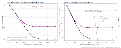
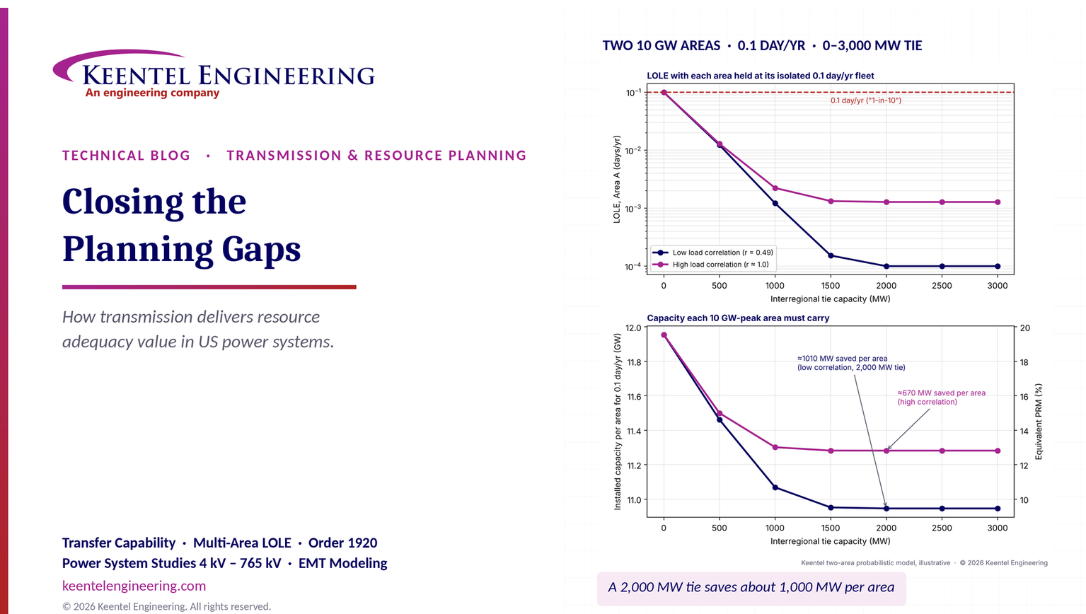
To make the value of transmission concrete, Keentel built a two-area probabilistic resource adequacy model. Each area has a 10,000 MW peak, a fleet of 100–600 MW thermal units with forced outage rates of 4–6%, and a year of daily peak loads with seasonal shape and weather variation. Each area alone needs about 11,955 MW of installed capacity — a 19.6% planning reserve margin — to meet a loss-of-load expectation (LOLE) of 0.1 day per year. Keentel then connected the two areas with a tie of 0 to 3,000 MW and asked how much capacity each area really needs.

Figure 1. Keentel's two-area probabilistic model. Left: LOLE in Area A when each area keeps its isolated 0.1 day/yr fleet and a tie of increasing capacity is added. Right: installed capacity each 10 GW-peak area must carry to meet 0.1 day/yr, with the equivalent planning reserve margin on the right axis. Results are illustrative.
| Tie capacity | LOLE with isolated fleet, low load correlation | LOLE, high load correlation | Capacity needed per area, low correlation | Capacity needed per area, high correlation |
|---|---|---|---|---|
| 0 MW | 0.099 day/yr | 0.099 day/yr | 11,955 MW (PRM 19.6%) | 11,955 MW (PRM 19.6%) |
| 500 MW | 0.012 | 0.013 | 11,462 MW (14.6%) | 11,500 MW (15.0%) |
| 1,000 MW | 0.0012 | 0.0022 | 11,069 MW (10.7%) | 11,301 MW (13.0%) |
| 2,000 MW | about 0.0001 | 0.0013 | 10,946 MW (9.5%) | 11,282 MW (12.8%) |
| 3,000 MW | about 0.0001 | 0.0013 | 10,946 MW (9.5%) | 11,282 MW (12.8%) |
Three results stand out:
- A 2,000 MW tie cut each area's capacity need by about 1,000 MW when the two areas' peak loads were only moderately correlated (correlation coefficient about 0.5, with peaks shifted by about two months). Across both areas that is about 2,000 MW of capacity that never has to be built.
- Even with identical weather, the tie was worth about 670 MW per area. Generator forced outages are largely independent between regions, so sharing reserves helps even when loads peak together. Load diversity adds value on top of outage diversity.
- The benefit saturates. Beyond about 1,500–2,000 MW, more tie capacity adds almost no RA value in this model, because the binding events become ones where both areas are short at the same time. The first gigawatt of interregional transfer capability is worth far more than the fifth.
At an illustrative capacity cost of $100/kW-year, the 2,000 MW of avoided capacity in the low-correlation case is worth about $200 million per year — more than the roughly $135 million per year annualized cost of a $1.8 billion transmission project at 7% over 40 years. That comparison counts only resource adequacy, before any production cost, congestion or resilience benefits. It is exactly the benefit that today's separated processes tend to leave out.
Engineering review of common statements about planning integration
| Statement often heard | Keentel's check |
|---|---|
| "Resource planning uses a 20-year horizon, while transmission planning looks only 5–10 years ahead." | Historically true for reliability planning: NERC TPL-001-5.1 requires a near-term (years 1–5) and long-term (years 6–10) assessment. But FERC Order No. 1920 (May 2024) now requires transmission providers in FERC-jurisdictional regions to run long-term regional planning over a horizon of at least 20 years, with scenarios refreshed at least every five years. Compliance is phased in, and several regions received schedule extensions, so confirm the current status in each region. Non-jurisdictional areas, including most of ERCOT, follow their own processes. |
| "Economic and multi-value transmission studies are now required by Order No. 1920." | Partly. Order No. 1920 requires long-term scenarios, at least seven categories of factors, and the measurement of at least seven benefits, one of which is reduced loss of load probability or reduced planning reserve margin. It does not mandate a specific multi-value project category, a specific benefit-cost threshold or a specific cost allocation; regions and states retain discretion, and Orders No. 1920-A and 1920-B adjusted the state role. |
| "Transmission planning models ignore resource adequacy, and resource adequacy models ignore transmission." | A fair simplification. Nodal reliability models test deterministic contingencies at fixed dispatch and do not compute LOLE. Most RA models use one zone or a handful of zones with fixed transfer limits. Some RTOs do run multi-area RA models with internal limits — but transfer limits are inputs, not decision variables. |
| "The 1-in-10 standard is a NERC requirement." | Not nationally. A LOLE of 0.1 day per year ("one day in ten years") is an industry convention used by many RTOs and utilities. NERC assesses adequacy through its Long-Term Reliability Assessment and probabilistic assessments; one regional NERC standard requires a 0.1 day/yr analysis for planning reserve. States and RTO tariffs set the actual criteria, and many are moving toward additional metrics such as expected unserved energy (EUE). |
| "Transmission has an ELCC like a generator." | Not directly. Effective load carrying capability (ELCC) is a resource accreditation concept. Transmission's RA value appears as reduced PRM, higher import limits, or "tie benefits" counted toward reserve requirements. It can be expressed as equivalent firm capacity using the same probabilistic method, which is how Keentel quantified it above. |
| "Assumed caps on external assistance limit the value of new transmission." | Correct, and often for defensible reasons: neighbors may be short at the same time, imports may not be deliverable, and firm commitments may not exist. But a fixed cap applied regardless of new transmission means the model cannot see the value of that transmission. The cap should be derived from multi-area modeling of simultaneous scarcity, not assumed. |
| "When RA benefits are socialized, merchant transmission has no incentive." | Reasonable. If an RTO credits import capability to all load in a zone, a participant-funded or merchant line cannot capture the capacity value it creates unless the market offers a product for it, such as capacity import rights, accredited firm imports or contractual capacity deliverability. Cost allocation design matters as much as engineering. |
| The process diagram shows a linear flow from RA to resource planning to transmission. | Real planning should iterate. Transmission alternatives change the PRM and the least-cost portfolio; the portfolio changes the transmission need. Without feedback loops, each process optimizes against stale assumptions from the others. |
Five lessons
- Transmission is a resource adequacy resource. It shares reserves, captures weather and load diversity, and lets regions hold less capacity for the same reliability. It should be valued that way.
- The value is strongly nonlinear. The first few hundred megawatts of transfer capability between weakly correlated regions are worth the most. Studies that test only one large project, or only one tie size, miss the shape of the curve.
- Correlated extreme weather is the binding case. Winter storms that hit several regions at once — and correlated failures of gas supply and generating units in the cold — limit how much help neighbors can give. Multi-area models need correlated weather years and correlated outages, not just independent unit outages.
- Data and horizon alignment is the cheapest fix. Using the same load forecasts, resource assumptions and weather years in RA, IRP and transmission studies removes much of the inconsistency before any new model is built.
- Order No. 1920 creates the opening. Its 20-year horizon and its required "reduced loss of load probability or reduced planning reserve margin" benefit give planners a formal place to count RA value — if the RA and transmission teams actually exchange models and results.
Part B — Technical Guide: Closing the Planning Gaps
1. The vocabulary of resource adequacy
Resource adequacy is the ability of the electric system to supply aggregate demand and energy requirements at all times, accounting for scheduled and reasonably expected unscheduled outages of system components. It is a planning concept, measured probabilistically, and distinct from operating reliability (surviving the next contingency) and from transmission security (meeting NERC TPL performance requirements for specified contingencies).
1.1 Probabilistic metrics
| Metric | Definition | Units | What it captures |
|---|---|---|---|
| LOLE — loss of load expectation | Expected number of days (or periods) per year in which available capacity is less than load | days/yr | Frequency of shortfall days; the traditional "0.1 day/yr" target |
| LOLH — loss of load hours | Expected number of hours per year with a shortfall | hours/yr | Duration as well as frequency |
| EUE — expected unserved energy | Expected energy not served per year | MWh/yr | Magnitude; increasingly used for energy-limited systems |
| LOLEV — loss of load events | Expected number of distinct shortfall events per year | events/yr | Separates one long event from many short ones |
| Normalized EUE | EUE divided by annual energy | ppm or % | Compares systems of different size |
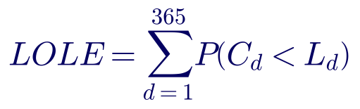
The daily LOLE is computed as the sum, over the days of the year, of the probability that available capacity falls below the daily peak load:

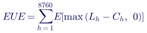
Expected unserved energy sums the expected shortfall over every hour:

Here C is available capacity (installed capacity minus random forced outages, plus energy-limited and weather-dependent output) and L is load. The 0.1 day/yr target is a long-standing convention, not a physical law; it corresponds to one loss-of-load day in ten years. Modern systems with high shares of solar, wind and storage can meet 0.1 day/yr while still carrying large EUE in a single long winter event, which is why many planners now examine several metrics together.
1.2 Planning reserve margin
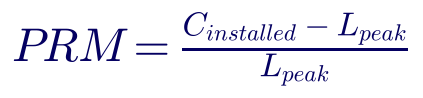
The planning reserve margin translates the probabilistic target into a simple capacity requirement:

Two conventions are in use. An installed-capacity (ICAP) PRM counts nameplate megawatts and must therefore be large enough to cover forced outages. An unforced-capacity (UCAP) or accredited-capacity PRM first derates each resource for its expected unavailability, so the required margin is smaller. Comparing PRMs across regions without checking the convention is a common mistake.

where EFORd is the equivalent demand forced outage rate. For variable and energy-limited resources, accreditation uses ELCC instead.
1.3 Effective load carrying capability (ELCC)
ELCC is the amount of perfectly reliable capacity that would provide the same reliability improvement as the resource being evaluated. It is found by adding the resource to the system, measuring the new LOLE or EUE, and then finding the amount of perfect capacity that achieves the same result.
- Average ELCC spreads the combined value of a resource class across all of its megawatts.
- Marginal ELCC measures the value of the next megawatt. As solar penetration grows, the net peak moves into the evening and the marginal ELCC of solar falls sharply. Storage shows a similar but slower decline as the net peak widens beyond its duration.
Several RTOs now use marginal or class-average ELCC for accreditation, and several are extending ELCC-style accreditation to thermal units using performance during the riskiest hours. Transmission does not receive an ELCC in these programs; its value appears through import limits, zonal requirements and the PRM itself.
Worked example 1 — LOLE from a capacity outage probability table
A small system has six identical 100 MW units, each with a forced outage rate of 5%. The probability that exactly k units are out is binomial:

| Units out | Capacity out | Capacity available | Probability |
|---|---|---|---|
| 0 | 0 MW | 600 MW | 0.73509 |
| 1 | 100 MW | 500 MW | 0.23213 |
| 2 | 200 MW | 400 MW | 0.03054 |
| 3 | 300 MW | 300 MW | 0.00214 |
| 4 or more | 400+ MW | 200 MW or less | 0.00009 |
The year's daily peaks are grouped into four bands: 30 days at 500 MW, 60 days at 450 MW, 120 days at 400 MW and 155 days at 350 MW. A shortfall occurs on a 500 MW day if two or more units are out (probability 0.03277), on a 450 MW day under the same condition, and on 400 MW and 350 MW days if three or more units are out (probability 0.00223).
| Fleet | Installed capacity | ICAP PRM on 500 MW peak | LOLE |
|---|---|---|---|
| 6 × 100 MW | 600 MW | 20% | 3.56 days/yr |
| 7 × 100 MW | 700 MW | 40% | 0.39 days/yr |
| 8 × 100 MW | 800 MW | 60% | 0.038 days/yr |
Small systems with large units need very large reserve margins to reach 0.1 day/yr, because losing one unit is a large fraction of the fleet. This is the first, and oldest, reason interconnection pays: pooling makes each unit a smaller share of the combined fleet. The same convolution, extended to hundreds of units in 50 MW steps, is the engine of Keentel's two-area model.
2. How resource adequacy is assessed in the United States
2.1 The assessment process
A modern RA study has five building blocks:
- Load. Hourly load shapes for many historical weather years (often 20–40 or more), scaled to the forecast year, with economic uncertainty and new large loads such as data centers layered on top.
- Thermal resources. Unit capacities, forced outage rates and, increasingly, temperature-dependent derates and correlated outages in extreme cold or heat.
- Variable resources. Wind and solar profiles synchronized to the same weather years as load, so the correlation between weather, load and renewable output is preserved.
- Energy-limited resources. Storage, hydro and demand response with their duration and use limits, dispatched in the model to minimize shortfall.
- Transmission. Usually a single zone, or a few zones linked by fixed transfer limits, plus an assumption about how much help neighboring regions can provide.
The model is solved by convolution (for simple systems) or by sequential Monte Carlo simulation, which samples thousands of years of random outages against the weather years and records every shortfall.
2.2 Correlated events change the answer
Two winter events changed how US planners think about adequacy. In February 2021 a prolonged cold-weather event in the central United States caused massive simultaneous outages of gas-fired, coal, nuclear and wind generation, much of it linked to freezing equipment and natural gas supply interruptions, and forced large-scale rotating outages in Texas. In December 2022 a fast-moving winter storm across the Eastern Interconnection produced very high forced outages, again concentrated in gas-fired generation, and rotating outages in parts of the Southeast.
Both events showed that outages are not independent random draws. They are correlated with temperature, with fuel supply and with each other — and they can hit several regions at once. For transmission planning this cuts both ways. It limits how much help a neighbor can give during a wide-area event, which is why RA studies cap external assistance. But it also shows the value of strong ties between regions whose weather extremes do not coincide, and of the ability to move power across long distances during regional emergencies.
2.3 RA programs in the RTOs (summarized)
| Region | How the RA requirement is set | How transmission enters |
|---|---|---|
| MISO | Seasonal Planning Resource Auction with zonal local reliability requirements; accreditation moving toward methods based on availability in high-risk hours | Capacity Import and Export Limits between zones derived from transmission studies |
| PJM | Reliability Pricing Model capacity auction; marginal ELCC accreditation for most resource classes in recent auctions | Capacity Emergency Transfer Limits and Objectives (CETL/CETO) determine constrained locational deliverability areas |
| SPP | Planning reserve margin requirement on load-responsible entities; requirements increased in recent years and a winter requirement added | Deliverability through the transmission service process |
| ERCOT | Energy-only market; reliability standard expressed in probabilistic terms with market and operational tools | Limited ties to other interconnections (DC ties); internal transmission planned through the regional planning process |
| West (outside CAISO) | Voluntary regional resource adequacy program with forward showing and operational sharing; CAISO has its own RA program | Participants must show transmission deliverability for counted resources |
| Southeast and other non-RTO areas | Utility IRPs and state commission reserve requirements | Utility transmission plans; firm transmission service for imports |
Program details change frequently; confirm current rules with each RTO before relying on them.
3. Resource planning and capacity expansion
3.1 What an IRP or capacity expansion study does
A capacity expansion model chooses which resources to build, retire and operate over a 15–25 year horizon to minimize total cost subject to load, policy and reliability constraints. Reliability enters as a constraint: accredited capacity must meet peak load times one plus the PRM, often with seasonal and local requirements. Transmission is usually represented as a "pipe-and-bubble" or transport model — zones connected by fixed flow limits with no Kirchhoff's voltage law, no contingencies and no losses beyond a simple factor.
3.2 Why the representation matters
A transport model is not wrong; it is coarse. Its weaknesses for this problem are specific:
- Transfer limits are inputs, fixed from the previous transmission cycle, so the model cannot trade transmission against generation.
- Interface limits in a real network depend on the dispatch pattern and on contingencies; a single number hides that.
- Capacity expansion uses accredited capacity values computed once, outside the model. If transmission changes the PRM or the ELCC of resources in each zone, the expansion model never sees it.
Worked example 2 — PRM and accreditation for a mixed portfolio
A 10,000 MW-peak area has the following resources. Thermal units are accredited at ICAP × (1 − EFORd); variable and storage resources at an illustrative ELCC.
| Resource | ICAP (MW) | Accreditation basis | Accredited capacity (MW) |
|---|---|---|---|
| Gas combined cycle | 6,000 | EFORd 5% | 5,700 |
| Gas combustion turbine | 3,000 | EFORd 8% | 2,760 |
| Coal | 1,200 | EFORd 10% | 1,080 |
| Solar | 2,000 | ELCC 20% | 400 |
| Wind | 1,000 | ELCC 15% | 150 |
| 4-hour storage | 1,000 | ELCC 85% | 850 |
| Total | 14,200 | 10,940 |
On an installed basis the PRM looks generous:
On an accredited basis the margin is only 9.4%. If the region's accredited requirement is, say, 12%, this area is about 260 MW short even though its installed reserve margin is 42%. The same area with access to more import capability could meet its target through the tie — but only if the RA study credits that import and the capacity expansion model knows it is available.
Worked example 3 — declining marginal capacity value of solar
Keentel modeled a simplified 10,000 MW system whose daily load peaks at 5 p.m. and a solar fleet whose output follows a midday arc ending around 7 p.m. The capacity value is measured as the reduction in net peak load per megawatt of solar added.
| Solar installed | Net peak (MW) | Net peak hour | Average capacity value | Marginal value of the last 1,000 MW |
|---|---|---|---|---|
| 0 MW | 10,000 | 5 p.m. | — | — |
| 1,000 MW | 9,535 | 5 p.m. | 46.5% | 46.5% |
| 2,000 MW | 9,286 | 6 p.m. | 35.7% | 24.9% |
| 3,000 MW | 9,164 | 7 p.m. | 27.9% | 12.2% |
| 4,000 MW | 9,164 | 7 p.m. | 20.9% | 0% |
Once the net peak shifts past sunset, more solar adds no capacity value in this simple model. Real ELCC studies, which consider many weather years and storage, show a similar shape. Transmission interacts with this effect: a tie to a region whose net peak occurs at a different hour can restore part of the lost value, because the combined system's net peak is broader and lower. A single-zone ELCC study cannot see that benefit.
4. Transmission planning in the United States
4.1 Reliability planning under NERC TPL-001-5.1
NERC Reliability Standard TPL-001-5.1 requires Planning Coordinators and Transmission Planners to assess their systems annually for a near-term horizon (years one through five) and a long-term horizon (years six through ten). The assessment uses steady-state, short-circuit and stability studies across a defined set of planning events, from single contingencies (P1) through extreme events, with stated performance requirements. Where violations are found, the planner must develop a Corrective Action Plan.
TPL-001 is deterministic. It asks whether the system meets performance requirements for specified contingencies at specified load and dispatch conditions. It does not ask how likely a capacity shortfall is, and it assumes that enough resources exist to serve the modeled load. That is why transmission reliability studies "ignore resource adequacy": it is not their job under the standard.
4.2 Regional and interregional planning under FERC Order No. 1000
FERC Order No. 1000 (2011) required each FERC-jurisdictional transmission provider to participate in a regional planning process that produces a regional plan, considers transmission needs driven by public policy requirements, and allocates the costs of selected regional facilities roughly commensurate with benefits. It also required interregional coordination procedures between neighboring regions. In practice, regional processes produced reliability, economic and policy-driven portfolios, while very few interregional projects were selected, because each region's own process had to find the project beneficial on its own terms.
4.3 Long-term regional planning under FERC Order No. 1920
FERC Order No. 1920, issued in May 2024 and modified on rehearing by Orders No. 1920-A and 1920-B, requires FERC-jurisdictional transmission providers to conduct long-term regional transmission planning. Its key elements are:
- A planning horizon of at least 20 years, with long-term scenarios developed and updated at least every five years.
- At least three long-term scenarios, including a scenario that reflects high-impact, low-frequency extreme weather and other events.
- At least seven categories of factors in developing the scenarios, including federal, state and local laws and policies, utility resource plans and load forecasts, trends in technology and fuel costs, retirements, generator interconnection requests and withdrawals, and corporate commitments.
- At least seven benefits to be measured when evaluating long-term projects: avoided or deferred reliability transmission facilities and aging infrastructure replacement; a benefit that can be characterized as either reduced loss of load probability or reduced planning reserve margin; production cost savings; reduced transmission energy losses; reduced congestion due to transmission outages; mitigation of extreme weather events and unexpected system conditions; and capacity cost benefits from reduced peak energy losses.
- A formal role for states in cost allocation for long-term regional facilities, with an engagement period.
- Requirements to consider right-sizing of replacement facilities and certain grid-enhancing technologies.
The second required benefit is the formal bridge this article is about. For the first time, FERC-jurisdictional regions must measure whether new long-term transmission reduces loss of load probability or reduces the planning reserve margin. Compliance filings and implementation schedules vary by region, and several regions received extensions; planners should confirm the status in each region.
4.4 Other national studies
- NERC's Interregional Transfer Capability Study, delivered in late 2024 at Congress's direction, assessed transfer capability between neighboring regions and identified roughly 35 GW of prudent additions to interregional transfer capability that would strengthen reliability under extreme conditions. It is an assessment, not a plan or a mandate, but it gives planners a consistent national baseline.
- The US Department of Energy's National Transmission Needs Study assessed historical and anticipated transmission needs and identified large benefits from additional interregional capacity, particularly between regions with different weather and resource patterns.
- RTO long-range portfolios — for example MISO's long-range transmission planning tranches, SPP's integrated transmission planning with new 765 kV facilities, PJM's regional transmission expansion planning, CAISO's transmission planning process and ERCOT's 765 kV plans — show that 765 kV and 500 kV AC backbones, and in some cases HVDC, are back on the planning agenda.
5. How transmission delivers resource adequacy value
Transmission does not generate a megawatt, but it changes how many megawatts each region must hold. Five mechanisms are at work.
| Mechanism | What happens | Where it shows up in RA studies |
|---|---|---|
| Outage diversity (reserve sharing) | Forced outages in two regions rarely coincide; a tie lets one region's spare capacity cover the other's outage | Lower LOLE for the same fleet; lower PRM; "tie benefit" |
| Load and weather diversity | Peaks occur on different days, seasons or hours in different regions | Larger LOLE reduction when load correlation is low |
| Resource diversity | Wind, solar and hydro output differ across regions; net peaks occur at different hours | Higher combined ELCC of variable resources; slower ELCC decline |
| Deliverability | Internal constraints prevent resources from serving load in a zone; new transmission removes the constraint | Higher capacity import limits; fewer local capacity requirements |
| Resilience to wide-area events | Long-distance ties connect regions whose extreme events are less correlated | Lower EUE in extreme-weather scenarios; Order No. 1920 extreme-event benefit |
5.1 The two-area model
In a two-area model, Area A experiences a shortfall only if its own margin is negative and Area B cannot make up the difference over the tie. With M as the available margin (capacity minus load) and T the tie capacity:
This simple model makes three implicit assumptions worth stating: Area B helps only from its own surplus (it does not shed its own load to help A), the tie is fully available when needed, and no internal constraints limit delivery inside either area. Real multi-area models add tie outage rates, internal zones, sharing rules and priority between areas.
Worked example 4 — Keentel's two-area result in detail
Keentel's model uses two areas with 10,000 MW peaks. Each fleet contains 100–600 MW units with forced outage rates of 4–6%, totaling 11,500 MW before tuning; firm capacity was then added or removed in both areas until each met 0.1 day/yr in isolation (11,955 MW, PRM 19.6%). Daily peak loads follow a seasonal curve with a weather-driven random component; the low-correlation case shifts Area B's seasonal peak by about 60 days and gives a daily-peak correlation of about 0.49, while the high-correlation case uses identical load shapes. The capacity outage probability tables are convolved exactly in 50 MW steps and the margin distribution of Area B is combined with that of Area A on each day.
Results are in Figure 1 and the Part A table. In the low-correlation case, the capacity each area must carry falls from 11,955 MW to 10,946 MW with a 2,000 MW tie:
In the high-correlation case the saving is about 673 MW per area, all from outage diversity. Most of the benefit arrives by 1,000–1,500 MW of tie capacity; beyond about 2,000 MW the curve is flat.
The practical meaning: if a region's RA study assumes a fixed 500 MW of external assistance, it has already captured only the steep first part of this curve and cannot see the value of the next 1,500 MW. If it assumes zero assistance, it overstates its capacity need by up to a gigawatt.
5.2 Quantifying the RA value of transmission: four methods
| Method | How it works | Strengths | Limitations |
|---|---|---|---|
| PRM reduction | Re-run the RA model with the new transmission and compute the lower PRM that still meets the target | Directly usable in IRPs and RTO requirements | Requires a multi-area model; sensitive to assistance assumptions |
| Equivalent firm capacity ("tie benefit") | Find the perfect capacity that would give the same LOLE improvement as the tie | Analogous to ELCC; easy to price at cost of new entry | Depends on the fleet and on neighbors' surplus |
| Import limit increase | Compute the change in capacity import limit or deliverability from transmission studies | Fits existing RTO zonal constructs | Deterministic; may not reflect probabilistic value |
| Avoided capacity cost in expansion | Co-optimize generation and transmission in a capacity expansion model with an RA constraint that depends on transfer capability | Captures the full trade-off | Computationally demanding; needs iteration with RA and power flow models |
Worked example 5 — does the RA value pay for the line?
Suppose the 2,000 MW tie in Worked example 4 is a 765 kV line costing $1.8 billion. At a 7% cost of capital over 40 years, the capital recovery factor is:

The annualized cost is $1.8 billion × 0.0750 ≈ $135 million per year, before operations and maintenance. At an illustrative avoided capacity cost of $100/kW-year:
| Case | Capacity avoided (both areas) | Avoided capacity cost | Ratio to annualized line cost |
|---|---|---|---|
| Low load correlation | about 2,018 MW | about $202 million/yr | about 1.5 |
| High load correlation | about 1,347 MW | about $135 million/yr | about 1.0 |
On RA value alone, the line roughly pays for itself in the high-correlation case and returns about 1.5 times its cost in the low-correlation case. Production cost savings, loss reductions, congestion relief and extreme-weather benefits come on top. These numbers are illustrative; real studies must use the regions' actual fleets, weather years, line costs and cost of new entry.
5.3 Why external assistance is capped
RA studies commonly cap the help a region can receive from its neighbors, sometimes at a fixed number of megawatts or at zero. The reasons are real:
- Simultaneous scarcity. During wide-area extreme weather, neighbors may be short at the same time.
- Firmness. Without firm contracts or firm transmission service, there is no guarantee that a neighbor's surplus will be offered.
- Deliverability. Internal constraints in either region may prevent surplus capacity from reaching the tie.
- Double counting. If every region counts its neighbors' surplus, the same megawatts may be counted twice.
The problem is not the cap itself but how it is set. A fixed cap applied in every scenario, regardless of the transmission in the model, removes the transmission's RA value by assumption. Keentel recommends deriving assistance limits from multi-area probabilistic modeling with correlated weather, and recomputing them when transmission changes.
6. Transfer capability: the link between the two worlds
The number that connects RA studies and transmission studies is transfer capability: how many megawatts can be moved from one area to another without violating thermal, voltage or stability limits under normal and contingency conditions. NERC defines first-contingency incremental transfer capability (FCITC) as the amount of power, above base-case flows, that can be transferred while respecting limits after the most limiting single contingency.
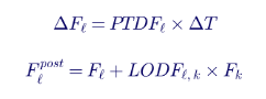
Linear sensitivity factors make the calculation transparent. The power transfer distribution factor (PTDF) gives the change in flow on a monitored element per megawatt of transfer; the line outage distribution factor (LODF) gives the share of an outaged line's flow that shifts onto the monitored element.

Worked example 6 — FCITC on a 345 kV interface
A 345 kV tie line between two areas has an emergency rating of 1,250 MVA (treated as MW here for simplicity). Its base-case flow is 400 MW and its PTDF for an A-to-B transfer is 0.45. A parallel 345 kV line carries 300 MW, has a PTDF of 0.35, and has an LODF of 0.55 onto the monitored line.
Without contingencies, the transfer limit set by this line would be:

After loss of the parallel line, the monitored line's base flow becomes 400 + 0.55 × 300 = 565 MW, and its effective sensitivity becomes 0.45 + 0.55 × 0.35 = 0.6425:

The first-contingency limit is about 1,070 MW — much lower than the 1,889 MW that a "pipe" model using the line's rating might assume. Real FCITC studies scan thousands of contingencies, include voltage and stability limits and model dispatch-dependent base flows. They also show why an RA study that uses a single transfer number from the previous planning cycle can be badly out of date when new lines, retirements or large loads change the flow pattern.
7. The seven gaps and how to close them
Keentel groups the integration problems into seven gaps. The first three concern regional planning; the last four concern interregional planning and markets.
| Gap | What goes wrong | How to close it |
|---|---|---|
| 1. Different horizons and objectives | RA studies often look one to five years ahead; IRPs 15–25 years; reliability transmission planning 1–10 years | Align on Order No. 1920's 20-year scenarios; share a common scenario set across RA, IRP and transmission teams; run RA studies for the same future years |
| 2. Different modeling methods | Nodal deterministic transmission models versus zonal probabilistic RA models | Build multi-area RA models whose zones and transfer limits come directly from nodal transfer studies; feed RA results back as reliability-driven benefits |
| 3. Different input data | Different load forecasts, weather years, resource lists and retirement assumptions | Maintain a shared planning database; use the same weather years for load, wind and solar in every study; document version control |
| 4. Interregional cost savings not explored | Each region evaluates its own needs; joint savings are invisible | Run joint multi-area RA and production cost studies between neighbors; test a range of tie sizes, not one project |
| 5. No best practice for RA value of transmission | PRM reduction, tie benefits and import limits are calculated inconsistently | Adopt a documented method (PRM reduction or equivalent firm capacity) with clear assumptions on assistance and firmness |
| 6. Fixed caps on external assistance | The model cannot see the value of new non-firm transmission | Derive assistance from multi-area modeling with correlated weather; update when transmission changes |
| 7. Socialized RA benefits | Merchant or participant-funded lines cannot capture the capacity value they create | Create mechanisms to credit firm deliverable imports to the party that funds them, such as capacity import rights, accredited firm imports, or contractual deliverability |
7.1 An integrated planning loop
Keentel recommends replacing the one-way chain in the typical process diagram with a loop:
- Step 1 — Common scenarios. Agree on 20-year scenarios, including load growth from data centers and electrification, retirements and policy, consistent with Order No. 1920.
- Step 2 — Candidate transmission. Define a set of transmission options with transfer capabilities computed by nodal FCITC analysis, including several sizes for each interregional interface.
- Step 3 — Multi-area RA. Compute LOLE, EUE and the required PRM for each transmission option using correlated weather years and derived assistance limits.
- Step 4 — Capacity expansion. Re-optimize the resource portfolio with the PRM and import limits from Step 3.
- Step 5 — Production cost and reliability testing. Test the combined portfolio for production cost benefits and TPL-001 reliability performance.
- Step 6 — Iterate. Repeat until the transmission plan and the resource plan stop changing materially.
The loop sounds heavy, but most of its value comes from the first iteration: discovering that the RA model's import assumptions and the transmission model's resource assumptions disagree.
7.2 Data and modeling checklist
- Use the same weather years for load, wind and solar across RA, IRP and transmission studies.
- Model temperature-dependent and correlated thermal outages, particularly in winter.
- Represent new large loads (data centers, industrial electrification) with realistic flexibility and ride-through assumptions.
- Derive zonal transfer limits from current nodal models, and record the dispatch and contingency that set each limit.
- Test several tie sizes to capture the nonlinear value curve.
- Report LOLE, LOLH and EUE together, and report the PRM convention (ICAP or accredited).
- Document every assumption about external assistance and its basis.
8. Cost allocation and incentives
Engineering can show that a line reduces capacity needs; cost allocation decides who pays and who benefits.
| Approach | How it works | RA implication |
|---|---|---|
| Beneficiary pays (regional allocation) | Costs allocated by measured benefits, often using a benefit metric formula | RA benefits must be measured to be allocated; Order No. 1920 makes this more likely |
| Postage stamp or load-ratio share | Costs spread across all load in the region | RA benefits are socialized; no individual party captures them |
| Participant funding | A generator, load or developer pays and receives the transmission rights | Works only if the market credits the funded capability toward the participant's capacity obligation |
| Merchant transmission (often HVDC) | Developer sells capacity on the line to customers | Needs a product that converts transfer capability into accredited capacity |
| State agreements | States negotiate allocation under Order No. 1920's engagement process | Can recognize RA value explicitly in the allocation formula |
A controllable HVDC link, for example a ±525 kV or ±600 kV voltage-source converter line between two regions, is attractive for capacity sharing because its flow can be scheduled and its deliverability is clear. But without a market mechanism that credits its capacity value to the party paying for it, much of that value flows to customers who did not fund it. Closing Gap 7 requires market design, not only engineering.
9. What engineers and planners should assess
- LOLE, LOLH and EUE for each transmission option, using a multi-area probabilistic model.
- The shape of the RA value curve versus tie or interface size, not a single point.
- Load, weather and resource correlation between the regions being connected, including extreme-weather years.
- First-contingency transfer capability of each option from nodal studies, including voltage and stability limits.
- External assistance assumptions, derived rather than assumed.
- PRM and accreditation impacts, stated in the region's convention.
- Avoided capacity cost versus annualized transmission cost, alongside production cost and resilience benefits.
- NERC TPL-001-5.1 performance of the final combined portfolio.
- Cost allocation and incentive design that matches who pays with who benefits.
Part C — Three Anonymous Case Studies
These composite case studies are based on the kinds of planning problems Keentel Engineering sees on US projects. Names, locations and identifying details have been changed or combined.
Case study 1 — A utility IRP that assumed zero help from its neighbors
Situation. A vertically integrated utility in the Southeast with a 9 GW summer peak and a growing winter peak was preparing its integrated resource plan. Its RA study modeled the utility as an island with zero external assistance, producing a required installed reserve margin of about 22% and a need for roughly 1,200 MW of new combustion turbines within six years. The utility had two 500 kV ties and several 230 kV ties to neighboring systems.
Analysis. Keentel reviewed the RA model and the transmission data. The neighbors' peaks were moderately correlated with the utility's in summer but much less so in winter, when the utility's morning peak came before a neighboring system's. Keentel built a three-area probabilistic model using the same 35 weather years for all three areas, with thermal outage rates that rose in extreme cold and with assistance limited by first-contingency transfer capability computed from the current nodal planning case. Assistance was capped during the coldest historical days to reflect simultaneous scarcity across all three areas.
Engineered solution. With derived assistance limits, the required reserve margin fell to about 17%, and the new-capacity need fell by about 400 MW. Keentel also evaluated an upgrade of one 230 kV tie to 345 kV, which raised winter transfer capability by about 600 MW and reduced the need by a further 150 MW at a fraction of the cost of new generation.
Outcome. The utility filed its IRP with a reduced combustion turbine build, a transmission upgrade in its regional plan and a documented method for external assistance that its commission staff accepted. The capacity savings were roughly four times the annualized cost of the transmission upgrade.
Case study 2 — An RTO zone where the import limit was out of date
Situation. A load zone inside a Midwest RTO was facing a local capacity shortfall after the announced retirement of a 700 MW coal unit. The zone's capacity import limit used in the RA program came from a transmission study two years earlier, before several 345 kV upgrades were completed and before a large data center campus requested 600 MW of new load at the zone's edge.
Analysis. A group of load-serving entities asked Keentel to examine whether the import limit was still valid. Keentel rebuilt the transfer study in the current nodal case, scanning all single and selected multiple contingencies, and found two offsetting effects. The completed 345 kV upgrades raised the thermal import limit by about 450 MW. But the new data center load, located near the limiting interface, shifted flows and created a new post-contingency overload on a 138 kV path that the previous study had never seen. The net change was an increase of about 150 MW — far less than the 450 MW a simple update would have assumed.
Engineered solution. Keentel identified a low-cost 138 kV reconductoring and a series reactor on a parallel path that together relieved the new limit, raising the net import capability by about 500 MW. The load-serving entities submitted the projects through the RTO's planning process with a documented RA benefit, and coordinated the data center's interconnection study so that its load was modeled consistently in both the RA and transmission studies.
Outcome. The RTO's next RA cycle used the updated import limit. The zone's local capacity requirement was met without emergency retention of the retiring unit, and the reconductoring was in service before the retirement.
Case study 3 — A merchant HVDC developer that needed a capacity product
Situation. A developer proposed a ±525 kV HVDC link of about 2,000 MW between a wind-rich region and a load-heavy region in another RTO. Production cost studies showed attractive energy arbitrage, but the developer's financing depended on selling capacity value to load-serving entities in the importing region. The importing RTO's capacity program treated external resources conservatively and capped external assistance in its RA study.
Analysis. Keentel built a two-region probabilistic model with 30 aligned weather years, including the major winter storms of recent years. The analysis showed that the regions' wind patterns and peak loads were weakly correlated on most of the risky days, and that the link could deliver about 1,300 MW of equivalent firm capacity to the importing region at 0.1 day/yr, falling to about 900 MW in the extreme-weather scenario when the exporting region was also stressed. Keentel also documented the converters' availability, the firmness of the exporting region's surplus, and the deliverability of the imported power from the converter station into the importing region's load centers through nodal transfer analysis.
Engineered solution. Keentel prepared an RA value report that the developer used to negotiate firm capacity contracts with two load-serving entities in the importing region, backed by firm transmission service and resource commitments in the exporting region. The report also supported the developer's request that the RTO recognize the contracted imports as accredited capacity.
Outcome. The developer secured contracts for about 900 MW of firm capacity — the extreme-weather value rather than the average — which was enough to reach financial close. The RTO later opened a stakeholder process on accreditation of firm external capacity backed by dedicated transmission.
Part D — 20-Question Technical FAQ
1. What is resource adequacy?
Resource adequacy is the ability of the power system to supply demand at all times, accounting for planned and unplanned outages of generation and other resources. It is measured probabilistically, usually with loss of load expectation (LOLE), loss of load hours (LOLH) and expected unserved energy (EUE), and translated into planning requirements such as a planning reserve margin.
2. What does "1-in-10" mean?
It is shorthand for a LOLE of 0.1 day per year: on average, one day in ten years with a capacity shortfall. It is a widely used industry convention rather than a single national NERC requirement. RTO tariffs, state commissions and some regional standards set the actual criteria, and many planners now also examine EUE and LOLH.
3. What is the difference between LOLE, LOLH and EUE?
LOLE counts expected shortfall days per year; LOLH counts expected shortfall hours; EUE measures the expected energy not served. A system with many short, shallow events and one with a single long, deep event can have the same LOLE but very different EUE. Systems with large amounts of storage and variable resources need all three.
4. What is a planning reserve margin?
It is the capacity a region must hold above its forecast peak load, expressed as a percentage of peak. It may be stated on an installed (nameplate) basis or an accredited (unforced or ELCC-based) basis. Accredited PRMs are smaller because each resource has already been derated for expected unavailability.
5. What is ELCC and why does it fall for solar?
Effective load carrying capability is the amount of perfectly reliable capacity that provides the same reliability improvement as a given resource. As solar grows, it pushes the net peak into evening hours when solar output is low, so each additional megawatt of solar does less to reduce the risk of shortfall. Keentel's simple example in Part B shows marginal capacity value falling from about 47% to zero as solar grows from 1 GW to 4 GW on a 10 GW system.
6. How does transmission provide resource adequacy value?
It lets regions share reserves when their generator outages do not coincide, capture load and weather diversity, use resources with different output patterns, and deliver capacity to constrained zones. All of these reduce the capacity each region must hold for the same reliability.
7. How large can the RA value of a tie be?
In Keentel's two-area model, a 2,000 MW tie reduced the capacity each 10 GW-peak area needed by about 1,000 MW when loads were moderately correlated, and by about 670 MW even when loads were identical. Real values depend on the fleets, the correlation of loads and extreme weather, and the deliverability of the tie.
8. Why does the value of transmission saturate?
Because the remaining shortfall risk comes from events when both regions are short at the same time. Once the tie is large enough to move all of one region's available surplus, more capacity does not help. That is why planners should test several sizes rather than one project.
9. Does Order No. 1920 require planners to count the RA value of transmission?
It requires FERC-jurisdictional regions to measure at least seven benefits for long-term regional transmission, including a benefit that can be characterized as reduced loss of load probability or reduced planning reserve margin. How the benefit is measured and how it affects selection and cost allocation are left largely to regional processes. Confirm each region's compliance status.
10. What planning horizon does Order No. 1920 use?
At least 20 years, with long-term scenarios developed at least every five years. NERC TPL-001-5.1 reliability assessments continue to cover the near-term (years one to five) and long-term (years six to ten) horizons.
11. Why do RA studies cap external assistance?
Because neighbors may be short at the same time, because surplus may not be firm, because internal constraints may block delivery, and to avoid counting the same megawatts twice. The issue is that fixed caps hide the value of new transmission. Assistance should be derived from multi-area modeling and updated when the network changes.
12. What is a capacity import limit?
It is the maximum amount of capacity that a zone can import for resource adequacy purposes, typically derived from transmission transfer studies. RTOs use import limits, or related constructs such as capacity emergency transfer limits, to decide how much of a zone's requirement can be met from outside the zone.
13. What is FCITC?
First-contingency incremental transfer capability: the additional power that can be transferred from one area to another above base-case flows while respecting thermal, voltage and stability limits after the most limiting single contingency. Keentel's worked example shows a 345 kV interface whose transfer limit falls from about 1,890 MW to about 1,070 MW once a parallel line outage is considered.
14. Why do capacity expansion models use "pipe-and-bubble" transmission?
Because nodal power flow with contingencies is too computationally heavy to embed in a 20-year optimization. The simplification is reasonable, but the zonal limits must come from current nodal studies and should be updated as the network and resource mix change.
15. How did recent winter storms change resource adequacy planning?
They showed that generator outages are correlated with extreme cold and with fuel supply, and that wide areas can be short at the same time. Planners now model temperature-dependent outages, use more weather years, emphasize winter risk and set accreditation based on performance in high-risk hours.
16. Can transmission replace generation entirely for resource adequacy?
No. It can reduce the amount of capacity each region needs and help deliver surplus where it is needed, but the interconnected system still needs enough total capacity. Transmission is most valuable when it connects regions whose risky hours differ.
17. How should HVDC links be treated in RA studies?
As controllable ties with defined capacity and availability, including converter outage rates. Their controllability makes deliverability easier to demonstrate, but the exporting region's surplus must still be available during the importing region's risky hours, and the importing region's internal network must be able to carry the power from the converter station.
18. Who benefits when RA value is socialized?
All load in the region shares the benefit through lower capacity requirements, regardless of who paid for the line. That is fair for regionally planned projects but discourages merchant and participant-funded transmission unless the market offers a way to credit the capacity value to the funding party.
19. What data should RA, IRP and transmission teams share?
The same load forecasts, including new large loads; the same resource lists and retirement dates; the same weather years for load, wind and solar; transfer limits from current nodal studies; and documented assumptions on external assistance and accreditation.
20. How can Keentel help?
Keentel performs nodal transfer capability and contingency studies, builds multi-area resource adequacy models, supports IRP and Order No. 1920 benefit analyses, and prepares interconnection and NERC compliance studies, so that the RA, resource and transmission assumptions in a client's plans are consistent.
Keentel Services, References and Contact
How Keentel Engineering Helps
Keentel Engineering supports utilities, RTO stakeholders, developers, large-load customers and state agencies at the point where resource adequacy, resource planning and transmission planning meet.
- Transfer capability studies. Nodal FCITC and import-limit analyses at 69 kV through 765 kV, with thermal, voltage and stability limits, to give RA and capacity expansion models defensible transfer numbers.
- Multi-area resource adequacy modeling. Probabilistic LOLE, LOLH and EUE studies with aligned weather years, correlated outages and derived external assistance.
- Transmission RA value and benefit-cost analysis. PRM reduction, equivalent firm capacity and avoided capacity cost analyses, structured to support Order No. 1920 long-term benefit measurement.
- IRP and planning support. Review of utility IRP and RTO planning assumptions for consistency between load, resource and transmission data.
- Interconnection and large-load studies. Generator interconnection studies under Order No. 2023 and large-load (data center) interconnection studies that feed consistent assumptions into planning models.
- HVDC and backbone transmission studies. Steady-state, stability and EMT studies for 500 kV and 765 kV AC and HVDC interregional options.
- NERC compliance. TPL-001-5.1 assessments, MOD-032 data and FAC-related support for Planning Coordinators and Transmission Planners.
Why Clients Choose Keentel
- We work across the silos. Our engineers understand nodal transmission studies, probabilistic RA models and capacity expansion, and we connect them.
- US standards fluency. NERC TPL and MOD standards; FERC Orders No. 1000, 1920 and 2023; RTO capacity constructs.
- Power system studies from 4 kV to 765 kV, including EMT modeling for HVDC and inverter-based resources.
- Transparent methods. Every assumption on assistance, accreditation and transfer capability is documented so regulators and stakeholders can follow it.
- Responsive senior engineers who stay with the project from scoping through regulatory filings.
Talk to Keentel Engineering
Is your resource plan built on transmission assumptions from the last planning cycle — or your transmission plan blind to the capacity it could save? Keentel Engineering can help you quantify the resource adequacy value of transmission and close the planning gaps.
- Phone: (813) 389-7871
- Email: contact@keentelengineering.com
- Book a 15-minute call: calendly.com/keentel-engineering/15min
- Web: keentelengineering.com
References
- FERC Order No. 1920, Building for the Future Through Electric Regional Transmission Planning and Cost Allocation, 2024; Orders No. 1920-A and 1920-B on rehearing.
- FERC Order No. 1000, Transmission Planning and Cost Allocation by Transmission Owning and Operating Public Utilities, 2011.
- FERC Order No. 2023, Improvements to Generator Interconnection Procedures and Agreements, 2023.
- NERC Reliability Standard TPL-001-5.1, Transmission System Planning Performance Requirements.
- NERC Reliability Standard MOD-032, Data for Power System Modeling and Analysis.
- NERC, Interregional Transfer Capability Study, 2024.
- NERC, Long-Term Reliability Assessment and Probabilistic Assessment reports (annual).
- NERC, Glossary of Terms Used in NERC Reliability Standards (Transfer Capability, First Contingency Incremental Transfer Capability).
- FERC, NERC and Regional Entity staff reports on the February 2021 cold weather event and the December 2022 winter storm.
- US Department of Energy, National Transmission Needs Study, 2023.
- IEEE Power & Energy Society, Resource Adequacy Working Group publications on probabilistic adequacy metrics.
- R. Billinton and R. N. Allan, Reliability Evaluation of Power Systems, 2nd ed., Plenum Press, 1996.
- A. J. Wood, B. F. Wollenberg and G. B. Sheblé, Power Generation, Operation, and Control, 3rd ed., Wiley, 2014.
- RTO resource adequacy and transmission planning manuals (MISO, PJM, SPP, ERCOT, CAISO) — current editions.
Disclaimer
This article is provided by Keentel Engineering for general technical education. It is not engineering, legal or regulatory advice for any specific project or filing. The models, fleets, costs and case studies are illustrative or composite, and results for real systems depend on actual data, models and regulatory rules. FERC orders, NERC standards and RTO rules change, and their implementation varies by region; always confirm current requirements with the applicable regulator, RTO and transmission provider. Keentel Engineering accepts no liability for decisions made on the basis of this article without a project-specific engineering review.
© 2026 Keentel Engineering. All rights reserved. Written by Keentel Engineering.
| Office | Address | Phone |
|---|---|---|
| Head Office — Tampa | 400 N Ashley Dr STE #2600, Tampa FL 33602 | (813) 389-7871 |
| Austin | 5900 Balcones Drive STE 100, Austin TX 78731 | (512) 591-0752 |
| Sacramento | 1401 21st St Ste R, Sacramento CA 95811 | (916) 913-4524 |
| Baltimore | 306 W Redwood St STE 200, Baltimore MD 21201 | (410) 225-2181 |

About the Author:
Sandip "Sonny" R. Patel, P.E.
IEEE Senior Member · Founder & CEO, Keentel Engineering
In 1995, Sonny Patel earned his Electrical Engineering degree from the University of Illinois. But degrees don't build legacies — action does.
For three decades, he has worked the power industry from every side of the table: 16 years as a utility engineer at Exelon/Commonwealth Edison; generation leadership across hydroelectric, industrial steam turbine, and a 9 GW renewable fleet; NERC Regional Entity Senior Compliance Engineer and Audit Team Lead, auditing some of the nation's largest utilities; and testing and commissioning lead on equipment up to 765 kV — the very top of the North American grid.Utility. Generator. Regulator. Consultant. Few engineers have seen all four seats. Fewer still have sat in them.
His experience spans nuclear, hydro, conventional generation, renewables, oil and gas, mining — and today's data centers, where he is authoring a three-book series on data center design. He is a Licensed Professional Engineer in six states and a Licensed Electrical Contractor in Florida (Unlimited EC) — he doesn't just design the work; he's qualified to stand behind its execution.Today, as Founder and CEO of Keentel Engineering, Sonny leads a nationwide team of engineers delivering substation design, power system studies, NERC compliance, and commissioning — done right, coast to coast.Three decades. Every side of the table. One standard: accountable engineering.
Services

Let's Discuss Your Project
Let's book a call to discuss your electrical engineering project that we can help you with.

About the Author:
Sandip "Sonny" R. Patel, P.E.
IEEE Senior Member · Founder & CEO, Keentel Engineering
In 1995, Sonny Patel earned his Electrical Engineering degree from the University of Illinois. But degrees don't build legacies — action does.
For three decades, he has worked the power industry from every side of the table: 16 years as a utility engineer at Exelon/Commonwealth Edison; generation leadership across hydroelectric, industrial steam turbine, and a 9 GW renewable fleet; NERC Regional Entity Senior Compliance Engineer and Audit Team Lead, auditing some of the nation's largest utilities; and testing and commissioning lead on equipment up to 765 kV — the very top of the North American grid.
Utility. Generator. Regulator. Consultant. Few engineers have seen all four seats. Fewer still have sat in them.
His experience spans nuclear, hydro, conventional generation, renewables, oil and gas, mining — and today's data centers, where he is authoring a three-book series on data center design. He is a Licensed Professional Engineer in six states and a Licensed Electrical Contractor in Florida (Unlimited EC) — he doesn't just design the work; he's qualified to stand behind its execution.
Today, as Founder and CEO of Keentel Engineering, Sonny leads a nationwide team of engineers delivering substation design, power system studies, NERC compliance, and commissioning — done right, coast to coast.Three decades. Every side of the table. One standard: accountable engineering.
Leave a Comment
We will get back to you as soon as possible.
Please try again later.