Part A — Solar PV and Load Tap Changers at a Glance
Most distribution interconnection studies for solar photovoltaic (PV) plants still answer one question: at maximum PV output and minimum feeder load, does the voltage stay inside its limits? If the answer is yes, the plant is often judged technically acceptable.
That question matters, but it is not enough. The hardest conditions for a distribution feeder are frequently not the steady peak of generation. They are the minutes when generation is changing — when broken clouds sweep across a 20 MW plant and its output swings by 10 or 15 MW in less than a minute, again and again, for hours.
During those minutes, the feeder voltage moves with the PV output. The substation load tap changer (LTC) and any line step-voltage regulators see the voltage leave their bandwidth, wait out their time delays, and then move their taps. When the cloud passes, they move back. A plant that looked acceptable in a single load-flow snapshot can multiply the number of tap operations, push customers outside the ANSI C84.1 service-voltage range for short periods, and accelerate wear on equipment that the utility expected to maintain on a fixed schedule.
Keentel Engineering's position is simple:
An acceptable voltage profile at one operating point does not prove acceptable voltage regulation over time. When a PV plant interacts with tap changers, regulators or capacitor banks, the interconnection study should include a time-domain voltage assessment — a quasi-static time-series (QSTS) analysis — using the real regulator settings, realistic loads and realistic PV variability.
This guide explains why, in US engineering terms. It covers how PV changes feeder voltage, how US LTCs and regulators actually make decisions, how line-drop compensation and reverse-power modes can be fooled by distributed generation, what IEEE 1547-2018 smart-inverter functions can and cannot do, how QSTS studies are built, and which mitigations work. Worked examples and Keentel's own QSTS simulation make the points concrete.
The feeder used in this guide
Keentel Engineering uses one illustrative US feeder throughout.
| Item | Value |
|---|---|
| Substation | 115/34.5 kV, 30 MVA transformer, about 10% impedance, with an on-load LTC (±10% in 32 steps) |
| Feeder | 34.5 kV radial overhead feeder, 10 miles, 477 kcmil ACSR, about 0.2 + j0.6 Ω per mile |
| Loads | An industrial customer near mid-feeder and residential load along the line; 8 MW at 0.95 power factor at the light-load condition studied |
| Solar plant | 20 MW (AC), connected near the end of the feeder |
| LTC control | 123 V on a 120 V base (1.025 pu), 2 V bandwidth (±1 V), 45 s initial time delay, 5 s intertap delay, line-drop compensation set to a load center 5 miles out |
| Voltage criteria | ANSI C84.1 Range A service voltage, 114–126 V on a 120 V base |
What Keentel's analysis shows
Keentel built a one-second QSTS model of this feeder and ran six hours of a broken-cloud day. The PV profile includes realistic plant-level smoothing: a 20 MW plant spread over about 100 acres does not change output instantly when a cloud edge arrives.

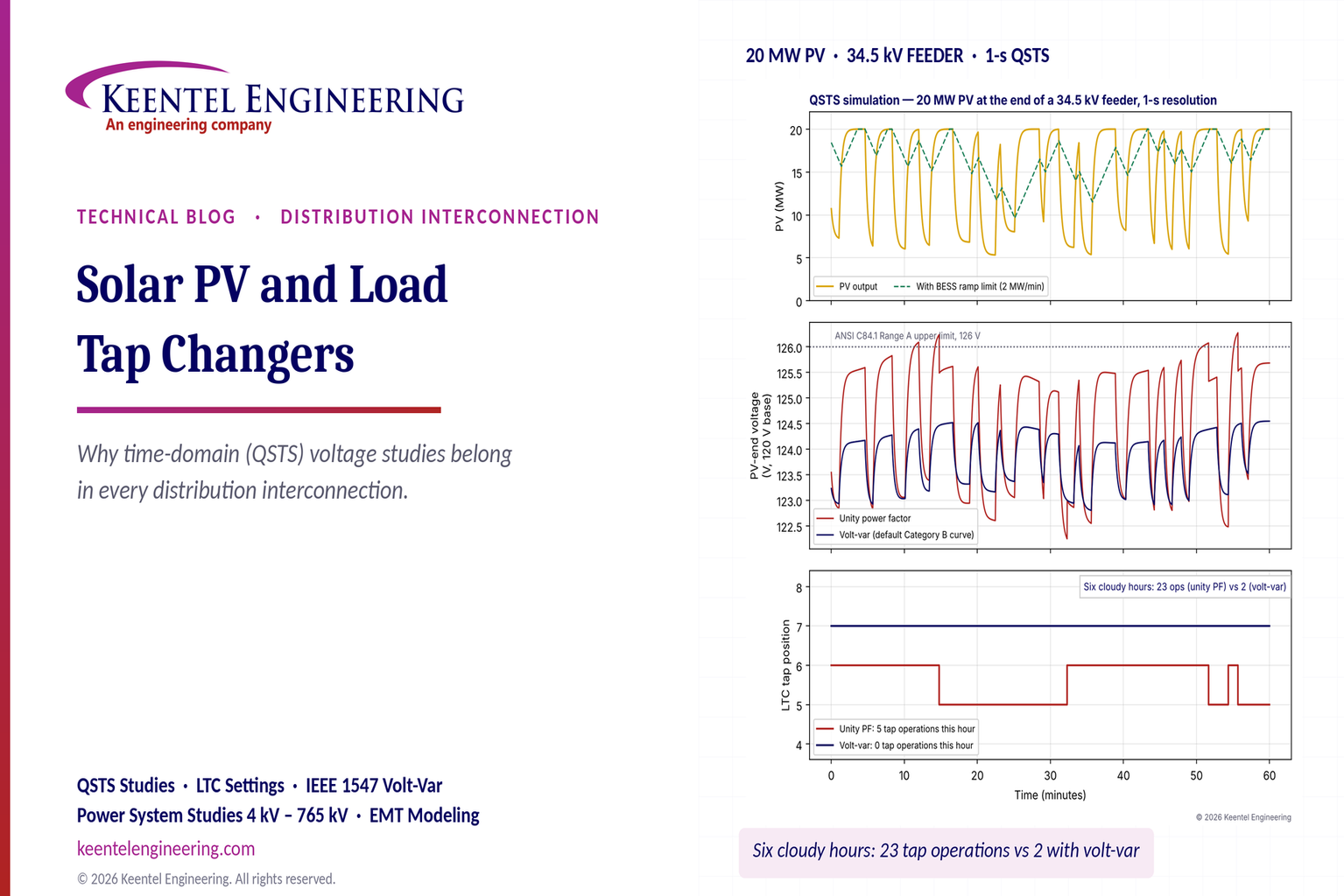
Figure 1. Keentel's QSTS simulation of a 20 MW PV plant at the end of a 34.5 kV feeder. Top: plant output over one cloudy hour, with and without a battery ramp-rate limit. Middle: voltage at the PV end of the feeder on a 120 V base, with the plant at unity power factor and with the default IEEE 1547-2018 Category B volt-var curve. Bottom: the substation LTC tap position for both cases.
| Case (six cloudy hours) | LTC tap operations | Time above 126 V at the PV end |
|---|---|---|
| No PV (same load) | 0 | 0 s |
| PV at unity power factor (base case) | 23 | 502 s |
| PV at unity power factor, LTC time delay raised to 90 s | 19 | 995 s |
| PV with default Category B volt-var | 2 | 0 s |
| PV with battery ramp-rate limit of 2 MW per minute | 3 | 41 s |
Four lessons stand out.
- Changing generation, not peak generation, drives tap operations. With steady load and no PV, the LTC did not move in six hours. The same load with a cloudy 20 MW plant produced 23 operations — roughly four per hour, or about 90 per day if the pattern persisted through a full cloudy day.
- Simply slowing the LTC is not a free fix. Raising the time delay from 45 s to 90 s cut operations by only about 17%, but nearly doubled the time customers spent above 126 V, because the LTC took longer to correct real overvoltages.
- Smart-inverter volt-var helps a great deal — if it is set and coordinated. The default IEEE 1547-2018 Category B curve absorbed up to about 4 Mvar during high output, flattened the voltage swings and reduced tap operations from 23 to 2. The trade-off is higher reactive flow and losses on the feeder, and an LTC that settles one step higher.
- Ramp-rate limiting with storage attacks the cause. A battery that limits the plant's net ramp to 2 MW per minute reduced tap operations to 3 — but it requires an energy-storage system sized for the job.
Engineering review of common statements about PV and tap changers
| Statement often heard | Keentel's check |
|---|---|
| "Consider a 20 MW plant on a 33 kV feeder fed from a 132/33 kV transformer." | These are not US voltages. The US equivalent is a 115/34.5 kV (or 138/34.5 kV) substation feeding a 34.5 kV distribution feeder. At 34.5 kV, 20 MW draws about 335 A. At 12.47 kV it would draw about 926 A — beyond the 600 A rating typical of US distribution feeders and switches — so a 20 MW plant at 12.47, 13.2 or 13.8 kV generally needs a dedicated express feeder or a higher voltage. |
| "Controller: setpoint 1.00 pu, deadband ±0.5%, 45 s initial delay, 5 s for successive steps." | Reasonable as a concept, but US controllers are set in volts on a 120 V base: a voltage level (often 120–124 V), a bandwidth (often 2–3 V total), a time delay (often 30–120 s) and, on many controls, an intertap delay. A ±0.5% band is 1% total, or 1.2 V — only just wider than one 0.75 V tap step. That is marginal once measurement error and regulator-to-regulator interaction are included; 2 V is the more common minimum. |
| The illustrative chart shows three tap-downs spaced 20–30 s apart. | With a 5 s successive delay, three steps would complete about 10 s after the first, not over a minute. The chart's spacing matches a control that re-times each step, or a sequential control with a longer intertap delay. The difference matters: QSTS models must use the actual timer logic of the installed control. |
| "Three tap steps moved the voltage about 1.5%." | One standard step is 0.625% (±10% in 32 steps), so three steps change the regulated-bus voltage by about 1.9%. A smaller change at the remote end is possible because PV output and feeder current also changed, but the step size itself should be stated correctly. |
| "A short PV dip does not cause a tap if the voltage returns within the deadband before the timer expires." | True for controls whose timer resets as soon as the voltage returns in band. Some controls use integrating timers that count down more slowly, or accumulate time across brief excursions. The same cloud can cause a tap on one control and not on another. |
| "Line-drop compensation (if used)." | Line-drop compensation is where PV causes the most surprising problems. It estimates the voltage drop to a load center from feeder current. When a PV plant exports near the end of the feeder, the substation current falls or reverses and the LTC lowers its output — even though the voltage drop to customers near the substation has not changed. This can cause low voltage upstream of the PV and must be checked explicitly. |
| "PV raises the feeder voltage to about 1.015 pu." | For a 20 MW plant at the end of a 10-mile 34.5 kV feeder, Keentel's load flow shows a rise of about 2.8% at unity power factor (about 3.4 V on a 120 V base). The rise depends heavily on the feeder's resistance, because distribution lines have low X/R ratios. |
| "Smart inverter volt-var may help, but must be coordinated." | Correct and important. In the US, IEEE 1547-2018 and UL 1741 SB define the functions and default curves, but the utility specifies the settings. A volt-var response faster than the LTC's time delay generally helps; a poorly chosen curve can fight the LTC or other plants. |
Five takeaways for developers, utilities and owners
- Ask for a time-domain study early whenever the plant is large relative to the feeder, is near the feeder end, or shares a feeder with LTCs, line regulators or switched capacitors.
- Model the controls as installed — voltage level, bandwidth, time delays, intertap logic, line-drop compensation and reverse-power mode — not as generic placeholders.
- Use realistic variability. One-minute or hourly PV data hide the cloud transients that drive tap operations. Use one-second irradiance data, scaled for plant footprint.
- Report regulation metrics, not just limits: tap operations per day, time outside Range A, rapid voltage change events, regulator reversals and losses.
- Design the mitigation with the utility: volt-var settings, power-factor schedules, ramp limits, regulator-setting changes or a dedicated feeder — and verify them in the same QSTS model.
Part B — Technical Guide: PV, Tap Changers and Time-Domain Voltage Studies
1. Why a single load-flow snapshot is not enough
A conventional distribution interconnection study runs a handful of power-flow cases: maximum PV at minimum load, maximum PV at peak load, and sometimes zero PV at peak load. Each case is a snapshot. The regulators and LTCs are usually allowed to settle at whatever tap position the solver chooses, and the result is a voltage profile that either passes or fails.
That method answers whether a steady operating point exists that keeps voltages in range. It does not answer:
- what voltage customers see before the regulators have moved, during the 30 to 120 seconds of time delay;
- how many times the regulators move per day as the plant's output varies;
- whether the regulators hunt — move up, then down, then up again — as clouds pass;
- whether line-drop compensation or reverse-power logic drives the regulator the wrong way;
- whether the plant's smart-inverter functions and the utility's regulators work together or fight each other;
- whether rapid voltage changes from cloud edges exceed flicker or rapid-voltage-change limits.
Those are time questions. Answering them needs a time-series model — the quasi-static time-series (QSTS) method described in Section 10.
What this means for owners and developers: a study that only checks maximum output can approve a plant that later generates complaints, regulator maintenance costs and curtailment requests. A time-domain check at the study stage is far cheaper than a retrofit after commercial operation.
2. How a PV plant changes feeder voltage
2.1 The voltage-change equation
For a radial feeder, the voltage change between the substation and a point where power P and reactive power Q are injected is approximately:

where R and X are the resistance and reactance of the feeder between the two points, V is the nominal voltage, and ΔV is in per unit when P and Q are in MW and Mvar, R and X in ohms and V in kV. Power flowing into the feeder from the PV plant raises the voltage; load drawn along the feeder lowers it.
On transmission lines, reactance dominates (X/R of 5 to 20), so voltage is controlled mostly by reactive power. Distribution lines are different. A 477 kcmil ACSR line at 34.5 kV has an X/R ratio of about 3, and smaller conductors or underground cable can be close to 1. Real power therefore changes distribution voltage directly — which is why every change in solar output shows up as a change in feeder voltage.
2.2 Worked example 1 — voltage rise from a 20 MW plant
The plant injects 20 MW at the end of a 10-mile, 34.5 kV feeder with R = 0.2 Ω/mi and X = 0.6 Ω/mi. Total feeder impedance is 2 + j6 Ω. At unity power factor:

A full load-flow solution, which accounts for the phase-angle shift along the feeder, gives a slightly smaller rise of about 2.8% — about 3.4 V on a 120 V base. If the plant instead operates at 0.95 power factor absorbing reactive power (Q = −6.57 Mvar):

The approximation says the rise almost vanishes; the full load flow shows the voltage settling about 0.6% below the substation voltage. Either way, absorbing reactive power at 0.95 power factor cancels almost all of the voltage rise — at the cost of drawing 6.57 Mvar through the feeder and substation transformer.
| Operating condition | Approximate ΔV | Load-flow ΔV | ΔV on a 120 V base |
|---|---|---|---|
| 20 MW, unity power factor | +3.4% | +2.8% | about +3.4 V |
| 20 MW, 0.95 power factor absorbing | about 0% | −0.6% | about −0.7 V |
The approximation is good enough for screening; the full load flow is required for design, because the approximation ignores the phase-angle term that becomes significant when P × X is large.
2.3 Worked example 2 — is 20 MW a distribution-scale plant?
Current for 20 MW at unity power factor is:

| Feeder voltage | Current for 20 MW |
|---|---|
| 12.47 kV | 926 A |
| 13.2 kV | 875 A |
| 13.8 kV | 837 A |
| 34.5 kV | 335 A |
Most US 12.47 kV to 13.8 kV feeders use 600 A switches, reclosers and regulators, and many feeder trunks are thermally limited to 400 to 600 A in summer. A 20 MW plant is therefore effectively a 34.5 kV-class interconnection, or a dedicated express feeder from the substation. On a 12.47 kV feeder, the practical limit for a plant sharing the feeder with customers is commonly in the range of 5 to 10 MW, set by thermal ratings, voltage rise and protection.
2.4 The feeder voltage profile
Along a feeder with load and no generation, voltage falls from the substation toward the end. The LTC is set high enough that the last customer stays above 114 V at peak load. Adding a large PV plant near the end reverses the slope on the downstream part of the feeder: voltage falls toward the load center and then rises toward the plant.
The worst overvoltage is usually at the plant at high output and light load. The worst undervoltage is usually at the end of the feeder at peak load with no PV — for example, when a thunderstorm drops the plant's output at 4 p.m. on a summer afternoon. Both extremes must be checked, and so must the transitions between them, because the regulators take time to respond.
3. The voltage limits that apply in the US
3.1 ANSI C84.1 service-voltage ranges
ANSI C84.1 defines the steady-state voltage ranges for US power systems. On a 120 V base:
| Range | Service voltage | Meaning |
|---|---|---|
| Range A | 114–126 V (0.95–1.05 pu) | Normal design range; voltages should be within this range most of the time |
| Range B | 110–127 V (about 0.917–1.058 pu) | Acceptable only infrequently and for limited durations; corrective action required |
Many utilities set tighter planning criteria, such as 116–125 V, to leave room for secondary and service-drop voltage drop and for measurement error. Utilization voltage at the equipment terminals is lower than service voltage because of the customer's own wiring.
The standard is written for steady-state voltage. It does not define how long a short excursion may last, which is why utilities and studies add time-based metrics such as seconds per day above 126 V.
3.2 Rapid voltage change and flicker
Cloud edges can change PV output by 50% or more in tens of seconds. The resulting voltage step is limited by two families of requirements:
- Rapid voltage change (RVC). IEEE 1547-2018 limits the rapid voltage changes a distributed energy resource (DER) may cause at the point of common coupling (PCC), with a tighter limit at medium-voltage PCCs than at low-voltage PCCs (on the order of 3% and 5%). Confirm the exact values and measurement method against the standard and the utility's requirements.
- Flicker. IEEE 1453 and IEEE 1547-2018 limit voltage fluctuations that cause visible light flicker, using the short-term (Pst) and long-term (Plt) flicker indices. PV cloud transients are usually too slow to create severe flicker, but repeated step changes and regulator operations can contribute.
3.3 Distribution interconnection standards
For distribution-connected plants, the governing technical standard is IEEE 1547-2018(with its 2020 amendment), with conformance testing under IEEE 1547.1-2020 and product certification under UL 1741 Supplement SB. IEEE 1547.7 describes distribution impact study methods, including time-series analysis. State interconnection rules and utility tariffs decide how these are applied; transmission-connected plants follow IEEE 2800-2022 instead.
4. US voltage regulation equipment
4.1 Substation load tap changers
A load tap changer (LTC) is built into the substation power transformer and changes its turns ratio under load. US substation LTCs typically provide ±10% regulation in 32 steps — 16 raise and 16 lower — of 5/8% each. Requirements for LTCs are covered by IEEE C57.131.
Two interrupter technologies dominate:
- Arcing-in-oil LTCs, which interrupt current in the diverter switch oil and generate carbon and wear with each operation.
- Vacuum LTCs, which interrupt in vacuum bottles, keep the oil much cleaner and typically allow many more operations between maintenance intervals.
4.2 Step-voltage regulators
Line step-voltage regulators are single-phase autotransformers with their own tap changer, installed in banks of three (or two, open-delta) along the feeder or at the substation. They follow IEEE C57.15 and also provide ±10% in 32 steps of 5/8%. Each has its own controller with the same settings as an LTC: voltage level, bandwidth, time delay and line-drop compensation.
4.3 Worked example 3 — step size and bandwidth on a 120 V base
One tap step is:

Three steps change the regulated voltage by 1.875%, or 2.25 V.
The bandwidth must be wider than one step, or the control may hunt: a single tap step could carry the voltage straight across the band and trigger a correction in the opposite direction. A common rule is:

Many US utilities use 2 V (±1 V) or 3 V (±1.5 V). A ±0.5% band — 1.2 V total — is only 1.6 times the step size and leaves little margin for potential-transformer error, voltage-sensing noise and the voltage changes caused by the PV plant itself.
4.4 Switched capacitor banks
Feeder capacitor banks switched on voltage, var, time or temperature also regulate voltage. A PV plant can change their switching pattern. Capacitor switching adds its own voltage step — often 1 to 3% — and its own operation count, so capacitor controls belong in the time-series model alongside the regulators.
5. How US regulator controls make decisions
5.1 The four core settings
Every LTC and step-voltage regulator control in US service works from the same four settings, all expressed on a 120 V base at the control's sensing input.
| Setting | Typical US range | What it does |
|---|---|---|
| Voltage level (set voltage) | 118–126 V; 120–124 V common | The target voltage at the regulation point |
| Bandwidth | 1.5–3 V total (±0.75 to ±1.5 V) | No action while the voltage stays inside this band |
| Time delay | 30–120 s; 45 s common for substation LTCs | How long the voltage must stay out of band before the first tap |
| Intertap delay (where provided) | 0–10 s | Time between successive taps once the control has decided to act |
Two further groups of settings — line-drop compensation and reverse-power mode — are where DER causes most problems. They are covered in Sections 6 and 7.
5.2 Timer behavior: the detail that decides tap counts
Controls differ in what they do when the voltage returns inside the band before the timer has expired:
- Instantaneous reset. The timer resets to zero as soon as the voltage returns in band. A 30-second cloud does not cause a tap on a control with a 45 s delay.
- Integrating timer. The timer counts down (often at the same rate) while the voltage is in band, so repeated short excursions can accumulate into a tap.
- Inverse-time delay. The delay shortens as the voltage deviation grows, so a large excursion is corrected quickly and a small one slowly.
Controls also differ in how they make successive taps:
- Sequential. After the first tap, the control waits the full time delay before the next tap. Three taps take three time delays.
- Time-integrating or " intertap " mode. After the first tap, successive taps follow at the intertap delay (for example 5 s) until the voltage is back in band.
- Voltage-averaging. The control calculates how many taps are needed and makes them in sequence after one time delay.
With a 45 s delay and 5 s intertap, three taps finish about 55 s after the voltage leaves the band. With sequential logic and a 45 s delay, the same three taps take more than two minutes. A QSTS model that uses the wrong timer logic will mis-predict tap counts and the duration of voltage excursions. Keentel models the actual control type and firmware settings, not a generic regulator.
5.3 Cascaded regulators
When a substation LTC and one or more line regulators are in series, their time delays are graded so the upstream device acts first. Common practice is to set each downstream regulator 15 s or more slower than the device upstream — for example 45 s at the LTC, 60 s at the first line regulator and 75 s at the second. Without grading, two regulators can both act on the same disturbance and overshoot, causing an extra round of corrections.
A PV plant downstream of a line regulator adds a third controller to this chain. If the plant's own voltage control acts on a time scale similar to the regulators', the three can interact. Section 9 explains how to set smart-inverter response times to avoid this.
6. Line-drop compensation and why PV confuses it
6.1 What line-drop compensation does
Line-drop compensation (LDC) lets an LTC or regulator regulate the voltage at a remote load center instead of at its own terminals. The control measures feeder current through a CT, multiplies it by a model of the line impedance (set as R and X in volts), and subtracts that estimated drop from the measured voltage:

The control then raises its output until the estimated load-center voltage reaches the voltage level. Heavier load means more current, more estimated drop and more boost, which is exactly what customers far from the substation need.
6.2 Worked example 4 — setting LDC in volts
The LTC regulates a 34.5 kV wye feeder. The load center is 5 miles out, with line impedance 1.0 + j3.0 Ω. The control uses a 600:0.2 A CT input (600 A rated primary) and senses line-to-neutral voltage through a 19,920:120 V potential transformer (ratio 166). The LDC settings in volts are:


With 15 MW of load at 0.95 power factor and no PV, feeder current is about 264 A and the control adds about 3.0 V of boost — matching the true drop to the load center.
6.3 What happens when the PV plant exports
Now add the PV plant beyond the load center. The LTC still sees only the current at the substation, which is load current minus PV current.
| PV output | Substation current | LDC boost | Actual drop to the load center |
|---|---|---|---|
| 0 MW | 264 A | 3.0 V | 3.0 V |
| 12 MW | 97 A | 1.8 V | 3.0 V |
| 20 MW | 118 A (now reverse real power) | 1.0 V | 3.0 V |
The load between the substation and the load center still draws the same current and still has the same voltage drop. But the LDC "thinks" the feeder is lightly loaded and lowers the voltage. Customers between the substation and the plant can see low voltage at exactly the moment the plant is producing the most power. When a cloud passes, the plant's output falls, substation current rises, and the LDC raises the voltage again — adding the LTC's response to every cloud.
Remedies include:
- reducing or removing the R and X settings and regulating closer to the substation;
- moving the PV plant to a dedicated feeder so it does not distort the load measurement;
- using a regulator control with DER-aware compensation, such as a feeder-head measurement that excludes the PV current, or a remote voltage sensor at the load center;
- checking the result in QSTS across the full year, not just at peak PV.
7. Reverse power flow and regulator modes
A large PV plant can push real power backward through a line regulator or even through the substation transformer. US regulator controls offer several reverse-power modes:
| Mode | Behavior when power reverses | Suitable when |
|---|---|---|
| Locked forward | Ignores reverse flow; keeps regulating the load side | Source always on the source side; small DER |
| Locked reverse | Regulates the source side only | Rare; special feeder configurations |
| Idle (neutral idle) | Stops tapping, or returns to neutral | Feeder ties where direction is uncertain |
| Bidirectional | Regulates whichever side is downstream of the measured power flow | Feeder ties and loops where the source changes |
| Co-generation (DG) mode | Keeps regulating the load side even when real power reverses | Radial feeders where DER causes reverse real power but the substation remains the voltage source |
| Reactive bidirectional | Decides direction from reactive power flow | Feeders with large DER and inductive source |
The common failure is a regulator left in bidirectional mode on a radial feeder. When the PV plant reverses real power, the control decides that the "source" is now the PV side and starts regulating the wrong terminal. Because the PV plant is not a stiff voltage source, each tap moves the voltage on the substation side only slightly, so the control can run its taps to the limit — the condition often called runaway. The fix is usually co-generation or reactive-bidirectional mode, chosen after a study of the actual feeder.
8. Tap operations, wear and maintenance cost
8.1 Why tap counts matter
Each tap change switches load current through the tap changer's contacts. For arcing-in-oil designs, every operation erodes contacts and adds carbon to the oil. LTCs and regulators are maintained on intervals set by time, operation count or both.
| Item | Indicative range (confirm with the manufacturer) |
|---|---|
| Typical substation LTC operations per day, no DER | Roughly 10 to 30 |
| Typical line-regulator operations per day, no DER | Roughly 20 to 80 |
| Arcing-in-oil LTC maintenance interval | Often tens of thousands of operations, or several years |
| Vacuum LTC maintenance interval | Often hundreds of thousands of operations, or longer time intervals |
| Mechanical life of the tap selector | On the order of one million operations |
If a PV plant doubles or triples daily tap counts, an arcing-in-oil LTC can reach its maintenance count years early. Utilities increasingly ask for tap-count impacts in interconnection studies and may allocate the resulting cost to the interconnecting customer, depending on state rules and tariffs.
8.2 Worked example 5 — the cost of extra tap operations
Keentel's QSTS model showed about four extra LTC operations per cloudy hour with the plant at unity power factor. Assume 120 cloudy days a year with six variable hours each:

Add a smaller number on clear days from morning and evening ramps — say 3,500 extra operations per year in total. If the LTC is maintained every 50,000 operations at an illustrative cost of $40,000 per maintenance:

That is modest for one LTC — but it is per regulator, it compounds with every PV plant on the feeder, and it ignores the larger cost of an LTC failure, which can take a substation transformer out of service for weeks. On an older arcing-in-oil LTC near the end of its maintenance cycle, the same extra operations may trigger an immediate inspection. The figures are illustrative; use the utility's own maintenance data.
9. Smart-inverter functions and coordination with regulators
9.1 The IEEE 1547-2018 voltage functions
IEEE 1547-2018 requires DER to be capable of several voltage-regulation functions. The utility decides which are enabled and with what settings.
| Function | What it does | Typical use |
|---|---|---|
| Constant power factor | Holds a fixed power factor, often absorbing (for example 0.95–0.98) | Simple, predictable; counters voltage rise at all output levels |
| Volt-var | Absorbs or injects reactive power as a function of local voltage | Responds only when voltage is high or low; reduces regulator activity |
| Watt-var | Sets reactive power as a function of real power output | Ties reactive absorption to output, independent of voltage |
| Volt-watt | Reduces real power when voltage is very high | Last-resort overvoltage protection; costs energy |
| Constant reactive power | Holds a fixed Mvar | Special cases |
DER are classed as Category A(reactive capability of at least 0.44 pu injecting and 0.25 pu absorbing, with a fixed default volt-var curve) or Category B(0.44 pu injecting and absorbing, with adjustable curves). Most utility-scale inverters meet Category B.
9.2 The default Category B volt-var curve
The default Category B volt-var curve, with reactive power in per unit of the DER's apparent-power rating, is:
| Voltage (pu) | Reactive power (pu) |
|---|---|
| 0.92 or below | +0.44 (injecting) |
| 0.98 | 0 |
| 0.98–1.02 | 0 (deadband) |
| 1.08 or above | −0.44 (absorbing) |
The default open-loop response time is 5 s, adjustable over a wide range (about 1 to 90 s for Category B). Utilities may change the curve points within the ranges the standard allows. Confirm current values against the standard and UL 1741 SB settings files.
9.3 Worked example 6 — volt-var output at high voltage
For a 20 MVA plant on the default curve, at local voltages above 1.02 pu:

| Local voltage | Q (pu) | Q for 20 MVA |
|---|---|---|
| 1.03 pu | −0.073 | −1.5 Mvar |
| 1.04 pu | −0.147 | −2.9 Mvar |
| 1.05 pu | −0.220 | −4.4 Mvar |
In Keentel's QSTS model, this response held the PV-end voltage below 124.6 V instead of about 126.3 V, and cut LTC operations from 23 to 2 over six cloudy hours.
9.4 Coordinating time scales
The rule of thumb is to keep the controllers on separate time scales:
- Inverter volt-var: seconds (a 5 s open-loop response is typical).
- Substation LTC: tens of seconds (30 to 60 s).
- Line regulators: graded behind the LTC (45 to 90 s and more).
- Switched capacitors: minutes.
The fast device then absorbs cloud-driven variability before the slower devices react, and the slow devices only respond to sustained changes such as load growth through the day. Problems arise when an inverter response is set very slow (tens of seconds) and competes with the LTC timer, or when several plants on the same feeder use steep curves that interact.
Two side effects must be checked:
- More reactive flow and losses. Absorbing reactive power raises feeder current and losses. In Keentel's model, the LTC settled one tap higher with volt-var active, because the extra reactive current increased the drop near the substation.
- Interaction with line-drop compensation. Reactive absorption changes the current the LTC measures, so LDC and volt-var must be evaluated together.
9.5 Power-factor schedules and volt-watt
A fixed absorbing power factor counters voltage rise in proportion to output and is simple to verify, but it absorbs reactive power even when the voltage is low. Watt-var schedules (for example, unity up to 50% output and then ramping to 0.95 absorbing at full output) are a common compromise. Volt-watt is usually reserved as a backstop, because it curtails energy.
10. Quasi-static time-series (QSTS) studies
10.1 What QSTS is
A QSTS study solves a sequence of power flows — one per time step — while keeping the state of every control between steps: regulator timers and tap positions, capacitor switching timers, inverter control states and battery state of charge. It captures how controls respond over time without the full electromagnetic detail of an EMT study. QSTS is described in IEEE 1547.7 and in published national-laboratory guidance on distribution DER studies, and is available in several QSTS-capable distribution analysis tools.
10.2 Choosing the time step and duration
| Study purpose | Typical time step | Typical duration |
|---|---|---|
| Tap-operation counts, regulator interaction | 1 s (or variable time-step) | Representative cloudy and clear days; ideally one year |
| Annual voltage and loss statistics | 1 min to 15 min | One year (8,760 hours) |
| Rapid voltage change and flicker screening | 1 s or faster | Worst cloudy days |
| Battery ramp-rate control sizing | 1 s | Worst cloudy days plus a statistical year |
A one-second, one-year QSTS run is 31.5 million power flows. Modern tools reduce run time with variable time steps (solving only when something changes), feeder reduction and parallel computing. Keentel typically runs a full year at one-minute resolution and the worst 20 to 30 days at one-second resolution.
10.3 Inputs that make or break the study
- Regulator and LTC controls as installed: set voltage, bandwidth, time delay, intertap delay, timer reset behavior, LDC settings, reverse-power mode, and starting tap positions.
- Capacitor controls: type, setpoints, delays and lockouts.
- Load profiles: feeder-head SCADA or AMI data, ideally allocated to customers by class, with the correct minimum-load days.
- PV variability: one-second irradiance data from a nearby site, converted to plant output with a spatial-smoothing filter scaled to the plant footprint; one-minute data underestimate tap operations because they average away short cloud events.
- Inverter functions: the actual volt-var, power-factor and ramp settings, including response times.
- Other DER on the feeder, including existing and queued plants.
- Transmission voltage variation at the substation high side, which also drives LTC operation.
10.4 Worked example 7 — Keentel's QSTS model
Keentel's model behind Figure 1 used:
- a 115/34.5 kV source with a 30 MVA, 10% substation transformer and an LTC (±10%, 32 steps);
- a 10-mile, 34.5 kV feeder in two 5-mile sections (1.0 + j3.0 Ω each), with 8 MW at 0.95 power factor at mid-feeder;
- an LTC set at 123 V, 2 V bandwidth, 45 s delay, 5 s intertap, with LDC to the mid-feeder load center and an instantaneous-reset timer;
- a 20 MW PV plant at the feeder end, with a synthetic broken-cloud profile (cloud shadows cutting output to 25–45% of clear-sky) and a 20 s plant-smoothing time constant;
- a slow ±0.4% variation in transmission voltage;
- a one-second time step over six hours, after a 10-minute initialization.
| Metric (six cloudy hours) | Unity PF | Volt-var | 90 s delay | BESS ramp limit |
|---|---|---|---|---|
| LTC tap operations | 23 | 2 | 19 | 3 |
| Highest PV-end voltage | 126.3 V | 124.6 V | 126.4 V | 126.1 V |
| Time above 126 V | 502 s | 0 s | 995 s | 41 s |
The model is deliberately simple, but it reproduces the behavior seen on real feeders: LDC and PV interaction, tap operations driven by cloud transients, and the trade-off between fewer operations and longer excursions when the time delay is raised.
10.5 Metrics to report
- tap operations per day for every LTC and regulator, with and without the plant;
- regulator reversals (a raise followed by a lower within a short window), which indicate hunting;
- time and number of events outside ANSI Range A and Range B at every customer node;
- rapid voltage change events at the PCC;
- capacitor switching operations;
- feeder losses and reactive power at the substation;
- PV energy curtailed by volt-watt or ramp control.
11. How time-domain studies fit US interconnection processes
Distribution interconnection in the US is governed mostly by state rules and utility tariffs. FERC's Small Generator Interconnection Procedures apply to FERC-jurisdictional interconnections, and many states have adopted similar fast-track screens and supplemental-review processes. State rules such as California's Rule 21, and utility hosting-capacity maps in several states, also shape what studies are required.
Common screens include penetration limits (for example, aggregate DER below 15% of peak line-section load) and minimum-load screens. When a plant fails a screen, the supplemental review or full study is the point at which a QSTS assessment belongs. Some utilities now require it explicitly for plants above a size threshold or on feeders with line regulators; others accept it when the developer offers it.
For a developer, a well-documented QSTS study can turn a "fail" into an approval with conditions — for example, a volt-var setting or a ramp limit — instead of an expensive upgrade.
12. Mitigation options
| Mitigation | How it helps | Trade-offs |
|---|---|---|
| Volt-var (IEEE 1547-2018) | Absorbs reactive power when voltage is high; reduces voltage swings and tap operations | Higher feeder current and losses; needs utility-approved settings |
| Fixed absorbing power factor or watt-var | Cancels much of the voltage rise in proportion to output | Absorbs vars even when not needed; losses |
| Battery ramp-rate control | Limits the rate of change of net plant output, attacking the cause of tap operations | Capital cost; energy and power must be sized for the worst cloud events |
| LTC and regulator setting changes | Wider bandwidth, adjusted time delays, timer-reset changes | Each change affects all customers on the feeder; may lengthen excursions |
| LDC retune or remote sensing | Removes the PV distortion of the load-current estimate | Requires engineering review; remote sensing needs communications |
| Reverse-power mode correction | Prevents runaway and wrong-terminal regulation | Must match feeder topology and switching |
| Relocating or adding regulators | Moves the regulation point to where it is needed | Capital cost, space and maintenance |
| Dedicated express feeder | Separates the plant from customer load and LDC measurement | Highest cost; often justified above about 10 MW at 12.47–13.8 kV |
| Distribution management systems (ADMS) with volt-var optimization | Coordinates regulators, capacitors and DER centrally | Utility system; long implementation time |
| Volt-watt or curtailment | Last-resort limit on overvoltage | Lost energy and revenue |
Keentel evaluates mitigation options in the same QSTS model used to find the problem, and reports the resulting tap counts, voltage statistics and lost energy for each option.
13. A practical study checklist
- Obtain regulator, LTC and capacitor control settings from the utility — not just nameplates.
- Confirm the control type and timer logic for each device.
- Build load profiles from feeder-head and AMI data, including the minimum-load days.
- Use one-second irradiance data and an appropriate plant-smoothing model.
- Include existing and queued DER on the feeder.
- Run snapshot cases first, then QSTS for representative and worst days, then a year.
- Report tap operations, reversals, Range A and B excursions, rapid voltage changes and losses, with and without the plant.
- Test mitigation options in the same model.
- Document every assumption so the utility can reproduce the results.
Part C — Case Studies
These composite case studies are based on the kinds of problems Keentel Engineering sees on US distribution interconnections. Names, locations and details have been changed or combined.
Case study 1 — A plant that passed its snapshot study and wore out a regulator
Situation. A 15 MW solar plant was connected near the end of a 34.5 kV rural feeder in the Southeast. The feeder had a substation LTC and one bank of line step-voltage regulators about 7 miles out. The interconnection study checked maximum output at minimum load and peak load with zero output, and found all voltages within ANSI Range A. The plant entered service at unity power factor.
Within a year, the utility's maintenance crews found that the line regulators' operation counters had risen from about 40 operations per day to more than 150 on summer days with afternoon storms. One regulator reached its contact-inspection count in under two years instead of the expected eight.
Analysis. Keentel built a QSTS model using one-second irradiance data from a nearby weather station, the utility's AMI load data and the regulators' actual settings. The model reproduced the measured counts within about 10%. It showed three causes:
- the regulators used a 30 s time delay and an instantaneous-reset timer, so every cloud lasting longer than 30 seconds caused a tap;
- the regulators' bandwidth was 1.5 V — only twice the 0.75 V step — so the voltage change from the plant's ramps often crossed the band in one step and caused a reverse tap shortly after;
- the substation LTC and the line regulators had the same 30 s time delay and both acted on the same events.
Engineered solution. Keentel recommended, and the utility and owner agreed to:
- enable the plant's volt-var function with the default Category B curve and a 5 s response time;
- widen the line-regulator bandwidth to 2 V and grade the time delays at 45 s for the LTC and 75 s for the line regulators;
- re-run the QSTS model to confirm Range A compliance at the most remote customers.
Outcome. Line-regulator operations dropped to about 50 per day on stormy days — close to the pre-plant level. No customer voltages left Range A in the follow-up year, and the utility added a QSTS requirement to its study guide for plants above 5 MW on regulated feeders.
Case study 2 — Line-drop compensation and low voltage near the substation
Situation. A Midwest utility connected a 10 MW solar plant to the end of a 13.2 kV feeder serving a small town. The substation LTC used line-drop compensation set for a load center in the town, about 3 miles from the substation. After the plant came online, residents on the first 2 miles of the feeder reported dimming lights and appliance trouble on sunny afternoons — the opposite of the overvoltage everyone had expected.
Analysis. Keentel reviewed the LTC control settings and SCADA data. On sunny afternoons, the plant's output nearly matched the feeder load, so the current measured at the substation fell to about 20% of its normal afternoon value. The LDC calculated almost no voltage drop and lowered the LTC output by about 3 V. Customers near the substation, still drawing normal load, saw service voltages around 112 V — inside Range B but outside Range A for hours at a time. The snapshot study had modeled the LTC as holding a fixed bus voltage and so had missed the problem entirely.
Engineered solution. Three changes were made:
- the LDC settings were reduced and the LTC voltage level raised by 1 V, which held the far end within limits without relying on current-based boost;
- a line regulator with co-generation reverse-power mode was added between the town and the plant, so the plant's voltage rise was regulated separately;
- the plant's power-factor schedule was set to 0.97 absorbing above 50% output.
Outcome. A 12-month QSTS run with the new settings showed all customers within Range A. Measured service voltages after the change confirmed the model, and the complaints stopped.
Case study 3 — Choosing between a battery and a dedicated feeder
Situation. A developer in the Southwest planned a 20 MW solar plant on an existing 12.47 kV feeder. The utility's initial study found that the plant would exceed the feeder's 600 A rating and require a new 4-mile dedicated feeder at a cost of several million dollars. The developer asked whether a battery could avoid the upgrade.
Analysis. Keentel confirmed that 20 MW at 12.47 kV is about 926 A — far above the feeder rating — so a battery alone could not make the full output deliverable. The real options were a smaller export limit on the existing feeder or a dedicated feeder. Keentel ran QSTS studies of two alternatives:
- a 10 MW export limit on the existing feeder, with the remaining output stored in a co-located battery and released in the evening;
- the full 20 MW on a new dedicated 34.5 kV feeder from an adjacent substation bus, with no shared customers.
For the shared-feeder option, the QSTS model showed that even at 10 MW the plant would add about 60 LTC operations per day on cloudy days, unless the battery also limited the net ramp rate to about 1 MW per minute. With ramp control and volt-var, operations stayed within 15% of the existing level.
Engineered solution. The developer chose a hybrid design: a 10 MW export limit on the existing feeder in the first phase, with a battery providing ramp control and evening shifting, and a reserved position for a dedicated 34.5 kV feeder in a later phase.
Outcome. The utility approved the first phase without a feeder upgrade, conditioned on the ramp-rate and volt-var settings demonstrated in the QSTS study. Field data from the first year confirmed tap-operation counts within the predicted range.