A Coordinated Electric System Interconnection Review—the utility’s deep-dive on technical and cost impacts of your project.
Challenge: Frequent false tripping using conventional electromechanical relays
Solution: SEL-487E integration with multi-terminal differential protection and dynamic inrush restraint
Result: 90% reduction in false trips, saving over $250,000 in downtime
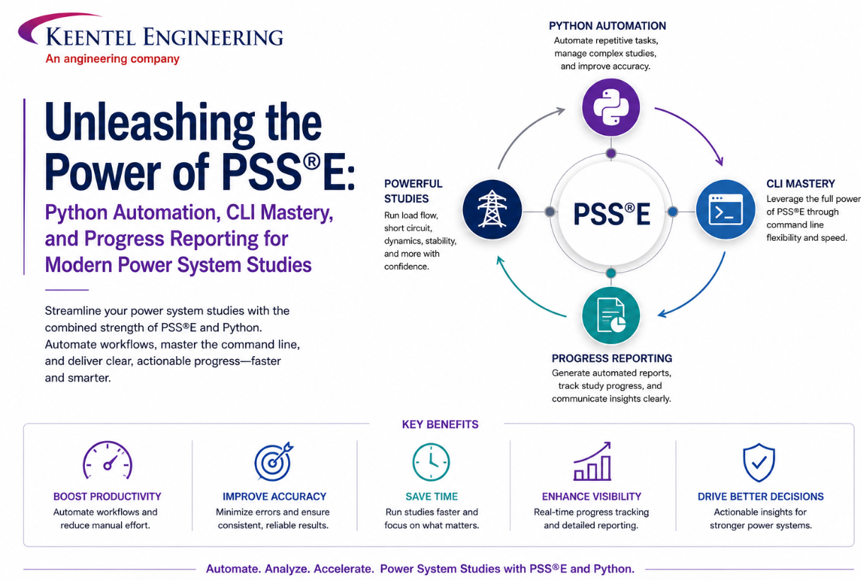
Unleashing the Power of PSS/E: Python Automation, CLI Mastery, and Progress Reporting for Modern Power System Studies
May 27, 2026 | Blog
Executive Summary
Modern power system studies demand more than manual point-and-click workflows. As transmission planning models become larger, interconnection queues become more complex, and regulatory scrutiny increases, engineers need repeatable, traceable, and highly automated study processes.
This technical guide from Keentel Engineering explores four foundational PSS/E productivity capabilities that enable engineering teams to scale their workflows while improving accuracy and auditability:
- External Python Integration
- Response File and Python Script Automation
- PSS/E Command Line Interface (CLI) Mastery
- Direct Progress Output (PDEV) Capture
The article also includes ten practical technical FAQs and three confidential client case studies demonstrating how these capabilities have delivered measurable value across utility, interconnection, and industrial reliability projects.
Part 1 — The Blog
Unleashing the Power of PSS/E with Python Automation
Siemens PSS/E remains the de facto standard for steady-state, dynamic, short-circuit, and contingency studies across transmission utilities, ISOs, IPPs, and large industrial customers. Yet most engineers still operate it the way they were taught a decade ago — point-and-click inside the graphical user interface (GUI), one case at a time, one report at a time. That works for a single study. It does not work when a queue cluster study has 47 generators, 14 contingency sets, and three sensitivity scenarios that all need to be re-run every time a model assumption changes.
At Keentel Engineering, our PSS/E practice is built on a simple premise: the GUI is the cockpit, but Python, the response file, the CLI, and the progress-output system are the autopilot. When these four capabilities are stitched together correctly, what used to take a week of manual clicking collapses into a script that runs overnight — and produces a fully traceable, auditable, regulator-ready record of every assumption, every solution attempt, and every iteration the solver took to converge.
This blog reviews four foundational capabilities every modern PSS/E user should master, organized exactly as we teach them to new analysts on our team.
1. Accessing PSS/E from Outside the GUI
The first level of PSS/E automation that most engineers encounter is the built-in recorder: start recording, click through a workflow, stop recording, and PSS/E writes a Python script that replays your steps. It is a friendly on-ramp — and it is also a ceiling. The recorder captures only what the GUI exposes. It cannot loop, cannot branch on solution status, cannot read external CSVs, cannot post to a database, and cannot orchestrate dozens of cases in parallel.
To get past that ceiling, PSS/E has to be driven from a Python interpreter that lives outside the PSS/E window. In that mode PSS/E becomes a library that your script imports, not an application you click. You keep the entire power and ecosystem of Python — pandas, NumPy, matplotlib, openpyxl, requests, multiprocessing — and you call PSS/E functions from inside it.
Which Python ships with which PSS/E?
One of the most common stumbling blocks for new automation users is mismatching the Python interpreter with the PSS/E version. PSS/E is tightly coupled to a specific Python build at install time, and using the wrong one is the most frequent reason an import psspy call silently fails.
| PSS/E Version | Bit Architecture | Bundled Python | Notes |
|---|---|---|---|
| v32 | 32-bit | Python 2.5 | Legacy installations, academic labs |
| v33 | 32-bit | Python 2.7 | Most widely deployed in industry |
| v34 | 32-bit / 64-bit | Py 2.7, 3.4, 3.9 | Transitional — multiple interpreters supported |
| v35 | 64-bit | Python 3.9 | Modern standard; pure 64-bit pipeline |
The Role of Energy Storage: Not Just How Much, But How It's UOur internal recommendation: for v33, use Python 2.7. For v34, Python 2.7 remains the most reliable bridge for external access, though Python 3 works for most workflows. For v35, use the bundled Python 3.9 — and standardise your team on it, because v35 is fully 64-bit and unlocks much larger cases without the 2 GB memory ceiling of the 32-bit world.
The mechanics of external access
Driving PSS/E externally requires three environment ingredients: the PSS/E binary directory has to be on the system PATH, the PSS/E Python library directory (the one containing psspy.pyc) has to be on PYTHONPATH or appended to sys.path at runtime, and the interpreter you launch has to match the bitness of PSS/E itself. Once those align, a working hello-world looks like this:
import syssys.path.append(r"C:\Program Files\PTI\PSSE35\35.4\PSSPY39")import psspyimport psse35psspy.psseinit(150000) # initialise with 150k-bus capacitypsspy.case(r"C:\studies\sample.sav")psspy.fnsl() # full Newton-Raphson power flowierr, mismatch = psspy.solved()print("Solved" if ierr == 0 else "Not converged")
Keentel field note
On a recent generator interconnection study with 38 sub-scenarios, switching from GUI execution to a single Python orchestrator reduced the wall-clock study time from 11 working days to 9 hours and eliminated three transcription errors that would have shown up in the deliverable to the ISO
Loss of Load Expectation, LOLE, Defined
LOLE measures the average number of hours per year in which available generation is expected to be insufficient to meet demand. A LOLE target of 0.1–0.3 hours per year is considered a high-reliability standard and represents what many advanced
power systems target today.
2. Recording Automation — Python Scripts vs. Response Files
PSS/E gives you two built-in recording formats, and the distinction between them matters. The response file (*.idv) is a flat list of PSS/E activity commands and their numerical arguments, written in the same dialect that the engine has used since the mainframe era. The Python script (*.py, *.pyc, *.pyw) is a sequence of psspy function calls written in modern Python syntax.
Both are produced by the same Start Recording → Stop Recording workflow under Input/Output Control. Both replay the same engineering operations. They diverge on what you can do after recording.
The response file (*.idv)
The IDV file is the simplest form of automation. It is human-readable, sequential, and runs without any Python interpreter on the host — PSS/E executes it natively. A recorded power-flow solve looks something like this:
FNSL,0,0,0,1,1,0,0,0RSOL,1PDEV,2,C:\studies\PF_summary.txt
Every comma-separated integer corresponds to one of the checkboxes or dropdown selections you made in the solution dialog: a 0 marks the default option, a 1 marks a non-default selection. (Programming starts at zero — the first option in any dialog is option 0, the second is 1, and so on.) That makes IDV files compact, version-controllable, and easy to diff in code review.
Where IDV shines:
- Repeatability — the same load flow with the same solution options, every time
- Audit trail — the file is the documentation of what was run
- Zero-dependency execution — any engineer with PSS/E can replay it, no Python install needed
- Speed — for linear, fixed workflows, IDV is the lowest-overhead format
Where IDV breaks down: it has no real control flow. You cannot loop over a list of generators, you cannot conditionally re-dispatch when the solution fails to converge, and you cannot read an external file to drive scenario inputs. For anything beyond a fixed recipe, you graduate to Python.
The Python script (*.py)
A recorded Python script is a sequence of psspy.* calls — psspy.fnsl, psspy.bsys, psspy.vchk, psspy.solv and so on — that maps one-to-one with the IDV activities but lives inside a real programming language. The same recorded workflow above, captured as Python, becomes something like:
import psspypsspy.bsys(0, 0, [0.0, 0.0], 1, [2], 0, [], 0, [], 0, []) # central area subsystempsspy.fnsl([0, 0, 0, 1, 1, 0, 0, 0])psspy.vchk(1, [0.95, 1.05]) # voltage limit check
Once it is Python, everything Python can do becomes available. The script can be parameterised, looped, wrapped in a function, called from a Jupyter notebook, scheduled by Windows Task Scheduler, or distributed across a multiprocessing pool that runs eight scenarios in parallel. It can pull bus dispatch from an Excel sheet, write violation summaries to a SQL database, and email the planner when the contingency study finishes.
When to choose which
Use response files (*.idv) for fixed, audited, regulator-facing workflows — final-deliverable load flow runs, sign-off cases, archival reproductions. Use Python scripts for everything that involves looping, branching, parameter sweeps, batch report generation, or integration with non-PSS/E tools. In our practice, the production pipeline is almost always Python; the IDV is the regulator-ready record we generate from it.
3. Mastering the PSS/E Command Line Interface
Long before Python integration existed, PSS/E was driven by a command line. That CLI is still alive inside the modern GUI — tucked into the Output Bar — and it remains one of the fastest ways to interrogate a case once you know the activity codes. The CLI accepts two dialects: native PSS/E response commands and Python statements. You toggle between them with a single click.
For day-to-day work, the response dialect is the workhorse. Want to open the bundled sample case without ever touching the File menu? Type the activity ID and the filename:
CASEsample.sav
The case loads with every option exactly as the .sav file specified. From there, the CLI exposes essentially the entire activity menu — every report, every check, every data-listing utility — by typing the three-to-five-letter activity code.
CLI commands every Keentel analyst memorises
| Activity | Purpose |
|---|---|
| CASE | Open a saved case (.sav) |
| FNSL | Full Newton-Raphson power flow solution |
| FDNS | Fixed-slope decoupled Newton-Raphson solution |
| RSOL | Re-solve from current solution state |
| VCHK | Voltage limit check across the working subsystem |
| LIST | List bus / branch / load / generator data |
| FIND | Locate a bus by number or name |
| RDCH | Read change file (incremental data updates) |
| PDEV | Direct progress output to file, printer, or report device |
| BSYS | Define or modify the active subsystem |
| AREA / OWNR / ZONE | Subsystem definitions by area, owner, or zone |
These activity codes are case-sensitive in some prompts and case-insensitive in others — a quirk that catches every new user once. The complete reference lives in the PSS/E CLI Guide installed under the documentation folder, organised into chapters by function (power flow data entry, dynamic simulation setup, program automation, and more).
The reason we still teach the CLI heavily — even in a Python-first world — is diagnostic speed.
When a converged case is suddenly mismatching by 50 MW, the fastest path to root cause is almost never to open a Python notebook. It is to type FIND followed by the suspect bus number, eyeball the data in the output bar, and have the answer in three seconds.
4. Capturing Solver Behaviour with Direct Progress Output (PDEV)
Every time PSS/E solves a power flow, the solver emits a stream of diagnostic messages — iteration counts, largest mismatches, transformer tap adjustments, switched-shunt actions, area interchange corrections, convergence warnings. By default, this stream flies past in the Progress tab and is gone. For a small radial network that solves in one iteration, that is fine. For a large meshed network in the middle of a software conversion, it is professional malpractice.
The Direct Progress Output activity — PDEV — redirects that diagnostic stream to a destination you control: a printer, a report device, or, most usefully, a text file.
Why progress capture matters
- Cross-software conversions. When a case is migrated from PSLF, DigSILENT PowerFactory, PSCAD, or another platform into PSS/E, the first solve almost always fails or converges to something physically unreasonable. The progress file is the forensic record that shows where the solver struggled — which transformers oscillated on tap, which areas refused to balance — and is the only practical guide for the engineer who has to make the case converge.
- Tap-adjust and switched-shunt diagnostics. On networks with many auto-transformers and switched shunts, the progress log records every tap movement and every shunt step. Comparing the log across runs is how we prove that a model change actually behaved as intended.
- Convergence triage on large meshed networks. Iteration-by-iteration mismatch trends tell you whether the case is genuinely close to a solution, stuck in a limit-cycle, or diverging. That distinction drives completely different remediation strategies.
- Auditability. For ISO-facing studies, the progress file becomes the contemporaneous record of how the solution was reached. It is the answer to the question every reviewer eventually asks: "prove this converged cleanly."
Setting up PDEV
From the GUI: Input/Output Control → Direct Progress Output. The dialog offers three destinations — printer, report device, or file — plus the option to append to an existing file. For most production work, choose File, give it an explicit path (we recommend a per-case subfolder, not the desktop), and set output lines per page to a high value (we use 9999) so multi-iteration runs are not broken across artificial page breaks.
From a Python script, the same redirect is one line:
psspy.progress_output(2, r"C:\studies\Case_A\progress.txt", [0, 0])psspy.fnsl([0, 0, 0, 1, 1, 0, 0, 0])psspy.progress_output(1, "", [0, 0]) # restore to default Progress tab
The first argument selects the destination (1 = report device, 2 = file, 6 = no output). Closing the redirect after the solve is important — leaving it open during subsequent activities pollutes the file with output you did not intend to capture.
Pro tip
On software-conversion projects, capture the progress output for every solve attempt, name the files by iteration number, and keep them all. The diff between progress_03.txt and progress_04.txt — i.e. what changed in the solver's behaviour after your last data fix — is the single highest-value piece of information on the entire project.
5. Putting It All Together — The Keentel Automation Stack
Read in isolation, each of the four capabilities above is useful. Stitched together, they become a production engineering workflow:
- Layer 1 external Python interpreter as the orchestrator (loops, branching, file I/O, parallelism)
- Layer 2 psspy calls or generated IDV files as the engine commands (the actual engineering work)
- Layer 3 CLI activities for interactive diagnostics and ad-hoc data queries
- Layer 4 PDEV-captured progress output as the forensic record of every solve
- Layer 5 pandas / openpyxl / matplotlib layered on top for reporting, dashboards, and stakeholder deliverables
This is the stack Keentel deploys on interconnection studies, transmission planning assessments, contingency screens, dynamic-stability prep work, and software migrations. It is also why a study that competitors quote in weeks, we quote in days — and deliver with a level of traceability that ISO reviewers consistently single out as exemplary.
If you are early in the PSS/E learning curve, start with the GUI recorder and the response file. Once recording feels limiting — and it will, faster than you expect — move to external Python. Layer in CLI fluency for diagnostics, PDEV for solver forensics, and the rest of the Python ecosystem for reporting. That progression is the same one we run every new engineer at Keentel through, and it is the foundation under every PSS/E deliverable we ship.
Part 3 — Confidential Case Studies
Confidentiality notice
The three case studies that follow are drawn from real Keentel Engineering client engagements. Client names, generator capacities, exact bus counts, ISO identifiers, and study dates have been altered or generalised to protect commercial confidentiality. The technical narrative, root causes, and engineering remedies are faithfully reproduced and reflect work delivered under NDA. Reproduction or redistribution outside the intended recipient is not permitted.
Case Study 1 — Generator Interconnection Cluster Study Automation
Client profile
Independent power producer with a portfolio of utility-scale solar and battery storage projects entering an ISO-administered cluster study queue. Six projects, aggregate nameplate approximately 1.4 GW, all interconnecting to a regional transmission network in the southwestern United States.
Engagement snapshot
| Service line | PSS/E modeling, automation, and interconnection studies |
|---|---|
| PSS/E version | v34 (64-bit) with bundled Python 3.9 |
| Network scale | ~28,000 buses, ~34,000 branches, ~3,800 generators |
| Study scope | Steady-state power flow + N-1 and N-1-1 contingency screening across 6 sub-scenarios per project |
| Original timeline (manual) | Estimated 14 working days using GUI workflow |
| Delivered timeline (automated) | 9 hours of compute + 2 days of engineering review |
| Confidentiality status | Delivered under NDA; project identifiers redacted |
The challenge
The client's prior consultant had been running each contingency scenario by hand inside the PSS/E GUI — opening the base case, applying the project's dispatch, running the contingency wizard, exporting violations to Excel, and repeating the process 36 times per project. With six projects and a fixed ISO submission window, the timeline was untenable, and three transcription errors had already been caught during internal QA on previous studies, each requiring a partial re-run.
The Keentel approach
We delivered a single Python orchestration framework, executed outside the PSS/E GUI, that ingested the project parameters from a master Excel workbook, looped over every project × scenario × contingency combination, captured solver progress output (PDEV) for every solve, and emitted a fully-formatted violation summary workbook plus a regulator-ready set of IDV response files documenting each run.
- Layer 1 Orchestration: a top-level Python script driving the entire 6-project pipeline with concurrent.futures, running 4 parallel PSS/E sessions on a 16-core workstation
- Layer 2 Engineering logic: psspy calls for case loading, dispatch redistribution, contingency application, FNSL solution, and violation extraction via psspy.abusreal
- Layer 3 Forensics: PDEV-captured progress files per scenario, archived for ISO submission
- Layer 4 Reporting: pandas-driven Excel output with per-project violation tables, sensitivity heatmaps, and a single executive-summary tab
Outcome
- Total study turnaround reduced from an estimated 14 working days to under 3 working days end-to-end
- Zero transcription errors flagged in internal QA or in the ISO's review
- Reusable framework retained by the client for the next queue cluster, reducing the marginal cost of future studies by approximately 70 percent
- ISO study group commended the deliverable's traceability — every violation was linked back to a specific progress file and IDV script
Case Study 2 — PSLF-to-PSS/E Migration for a Regional Utility
Client profile
Investor-owned transmission utility operating in a vertically-integrated market, migrating its transmission planning model base from GE PSLF to Siemens PSS/E to align with neighboring utilities and a regional planning entity. Approximately 18,000 buses in the base case, with seasonal peak and shoulder models maintained on a rolling basis.
Engagement snapshot
| Service line | PSS/E modeling, software migration, and convergence engineering |
|---|---|
| Source platform | GE PSLF — multiple seasonal cases |
| Network scale | ~18,000 buses, ~22,000 branches, ~1,900 generators across 7 areas |
| Critical issue | First-pass converted case diverged after 3 iterations with mismatches above 1,200 MW |
| Delivery | Fully converged seasonal model set with documented PDEV progress trail for each case |
| Confidentiality status | Delivered under NDA; utility and region redacted |
The challenge
The off-the-shelf PSLF-to-PSS/E conversion utility produced a syntactically valid PSS/E .sav file, but the case refused to converge. Initial mismatches exceeded 1,200 MW after the first FNSL iteration, and the solver oscillated rather than converging. The client had been blocked on this conversion for six weeks before engaging Keentel.
The Keentel approach
We treated the converged-case problem as a forensic engineering exercise built entirely on PSS/E's progress output. The workflow looked like this:
- Enable PDEV on every solve attempt with a unique, indexed filename — progress_001.txt through progress_054.txt by the time we converged
- Run a single iteration of FNSL with var limits ignored and tap adjustment locked, to capture the solver's view of the initial state without any internal corrections masking the underlying issues
- Parse the progress files with a small Python tool that flagged the largest contributing mismatches per area and per voltage class
- Triage the findings against a checklist of known conversion pitfalls — transformer tap convention sign flips, area interchange definitions, switched-shunt status, induction motor load model translation
- Iterate: apply a targeted data fix via psspy calls, capture the new progress file, diff against the previous run, repeat
Root cause
Three issues, found in this order: (1) auto-transformer tap conventions were inverted on a population of 230/115 kV transformers, producing voltage-control fight loops between adjacent transformers; (2) area interchange targets had not been transferred at all — every area was attempting to balance at zero net interchange against historical flows of several hundred megawatts; (3) a subset of switched shunts had been imported with non-zero step counts but in the 'unavailable' status, leaving the solver no reactive headroom in three key 345 kV substations.
Outcome
- All four seasonal cases converged cleanly within 6 to 9 FNSL iterations
- Total engagement duration: 4 weeks, against a 6-week block the client had already experienced with no progress
- Delivered a written convergence-engineering playbook keyed to PSLF-PSS/E migrations specifically, retained by the client's planning group as internal IP
- Full PDEV progress-file archive handed over as evidence of solution quality for internal model governance review
Case Study 3 — Confidential Industrial Microgrid Reliability Study
Client profile
Heavy-industrial facility with a captive on-site generation portfolio (gas turbines, steam turbines, and a battery energy storage system) interconnected to a host utility at a single 138 kV point of common coupling. Total facility load approximately 280 MW, with critical process loads that cannot tolerate sustained voltage excursions or frequency disturbances.
Engagement snapshot
| Service line | PSS/E modeling, contingency analysis, and industrial reliability studies |
|---|---|
| PSS/E version | v34 with Python 2.7 |
| Network scale | Detailed internal network (~340 buses) embedded in a regional model |
| Study scope | N-1 contingency screen + selected N-1-1 events + islanded operation feasibility |
| Critical question | Can the facility ride through loss of the utility tie and operate islanded for 4+ hours? |
| Deliverable | Reliability assessment + CLI-based diagnostic playbook for the facility's operations engineering team |
| Confidentiality status | Delivered under NDA; industry sector and location redacted |
The challenge
The client suspected — but had not quantified — that the loss of the utility tie under certain dispatch conditions would produce post-disturbance voltages outside the tolerance band of its variable-frequency drives, with the result that critical process equipment would trip before the gas turbines could pick up the dropped reactive support. The previous reliability study had been conducted purely in the GUI, was three years old, and reflected a generation portfolio that had since been expanded with the BESS.
The Keentel approach
We delivered the study in three layers, each adding traceability and shelf life:
- Power flow base — a Python automation that exercised the facility against 24 dispatch scenarios (base, BESS-charging, BESS-discharging, peak summer, off-peak winter, and so on), applied each of 47 N-1 contingencies, and captured PDEV progress output for every solve
- Diagnostic CLI playbook — a separate deliverable: a curated set of PSS/E response-file (.idv) scripts the client's own operations engineers could execute from the command line during real-time event reviews, without needing Python expertise. Each playbook covered a specific event class (tie loss, generator trip, busbar outage) and produced a standard one-page diagnostic report
- Islanded operation feasibility — a sequence of progressively-loaded power flows simulating the 4-hour islanded ride-through, with var support staged across the gas turbines and BESS, and progress output captured to demonstrate solver stability throughout the transition
Findings
- Under three specific dispatch conditions, loss of the utility tie produced bus voltages at the VFD bus that dipped below 0.92 pu for 1.4 to 2.1 seconds — within the trip envelope of the installed drives
- Adjusting the BESS dispatch logic to pre-emptively contribute reactive power on detected tie-loss reduced the worst-case excursion to 0.96 pu, well within tolerance
- Islanded 4-hour operation was demonstrated as feasible across all studied dispatch conditions, with a 9 percent reactive margin retained at the worst operating point
Outcome
- Client capital-deferred a proposed second utility tie that had been on the 5-year capital plan, on the basis of the demonstrated BESS-supported ride-through capability
- CLI playbook adopted as standing operating procedure for the facility's electrical engineering team — they now run post-event diagnostics in-house within 30 minutes of any disturbance, where previously they had to engage an external consultant
- Full PDEV-progress archive retained for the facility's insurance carrier as documented evidence of the reliability assessment
Closing — Talk to Keentel
Every engagement above started the same way: a conversation. If your team is wrestling with PSS/E productivity, stuck on a converted case that refuses to solve, drowning in cluster-study volume, or simply trying to build out an internal automation practice and not sure where to begin — that is exactly the conversation we want to have.
Keentel Engineering's PSS/E service line combines deep utility-grade modeling experience with modern Python-driven automation discipline. We have done the slow, painful learning curve so our clients do not have to repeat it.
Get in touch
To discuss a PSS/E modeling, automation, or convergence engineering need, contact the Keentel Engineering services team. All initial scoping conversations are conducted under mutual NDA. Engagement structures range from fixed-fee deliverables to embedded staff augmentation for utility planning groups.
Part 2 — 10 Technical FAQs
These are the questions our PSS/E team is asked most often by clients, peer reviewers, and engineers being onboarded. They distill the practical knowledge that experience teaches but textbooks do not.
Q1. My import psspy command fails with 'DLL load failed' or 'module not found'. What's wrong?
Almost always one of three things: (1) the Python interpreter you launched does not match the bitness of PSS/E — for example you are using 64-bit Python with a 32-bit PSS/E v33 install; (2) the PSS/E binary directory is not on the system PATH; or (3) the PSSPY directory (PSSBIN, PSSPY27, PSSPY39 depending on version) is not on sys.path. The fix is to launch the correct interpreter for your PSS/E version (Python 2.7 for v33, Python 3.9 for v35), append the PSSPY directory to sys.path before the import, and confirm the binary directory is in PATH. Set the PSSE_PATH environment variable to make this permanent across reboots.
Q2. Should I record a Python script or a response (IDV) file when automating a workflow?
Use IDV for fixed, deterministic, regulator-facing workflows where the value is reproducibility and zero dependencies — anyone with PSS/E on their machine can replay it without Python installed. Use Python when the workflow needs control flow: loops over scenarios, conditional re-dispatch, reading inputs from Excel or CSV, parallel execution, or any integration with tools outside PSS/E. In our practice, production work is Python, and an IDV is generated from the Python pipeline as the regulator-ready archive copy.
Q3. What does an activity argument like [0, 0, 0, 1, 1, 0, 0, 0] actually mean in fnsl?
Each integer is one of the option fields exposed in the Power Flow Solution dialog, in the order they appear. A 0 means the default option for that field; a non-zero value means a non-default selection (tap adjustment locked, var limits ignored, area interchange disabled, and so on). The PSS/E API Reference lists the meaning of each position for every psspy function. We strongly recommend wrapping these calls in named helper functions inside your project — fnsl_locked_taps() is far more readable in a code review than a bare integer list.
Q4. How do I reliably capture the solver's progress messages to a file from a Python script?
Call psspy.progress_output(2, filename, [0, 0]) before the solve and psspy.progress_output(1, '', [0, 0]) immediately after. The 2 selects file output, the [0, 0] controls whether to append. The most common mistake is forgetting to restore the default after the solve, which causes every subsequent activity — even unrelated ones — to keep writing to the same file. For multi-scenario runs, open a fresh progress file per scenario and name it deterministically.
Q5. My case converges in the GUI but won't converge when I run the same script externally. Why?
Three causes account for the majority of cases: (1) the script does not load the same auxiliary data the GUI loaded — bus subsystem definitions, switched-shunt status, dynamics data — because those state items live in memory, not in the .sav file; (2) the solution options differ subtly, often because the GUI remembered a setting you changed manually and the script uses defaults; (3) the script issues the solve before all data updates have been committed. The cure is to explicitly set every solution option in the script and to inspect the progress output side-by-side with a known-good GUI run.
Q6. What's the right way to handle voltage-violation reporting across hundreds of buses?
Use psspy.vchk to run the check, redirect progress output to a file with PDEV, and parse the resulting text into pandas in the same script. Better: skip parsing entirely and use psspy.abusint / psspy.abusreal to pull bus numbers and voltages directly into Python lists, then build the violation report in pandas. The direct API route avoids the brittleness of text parsing and produces a DataFrame you can pivot, sort, group by area, and export to Excel in two more lines.
Q7. Can I run PSS/E solves in parallel from a single Python process?
Not in the same process — psspy is stateful and a single Python process holds one PSS/E session. You can absolutely parallelise across processes using multiprocessing or concurrent.futures.ProcessPoolExecutor, with each worker launching its own PSS/E session against a different case copy. Be careful with file-locking on shared output directories and license-server seat limits. Our typical pattern is one worker per physical core, each writing to a worker-specific subdirectory, with a final aggregation step in the parent process.
Q8. What's the difference between FNSL and FDNS, and when should I use each?
FNSL is the full Newton-Raphson method — it builds and factorises the full Jacobian at every iteration and converges quadratically once near the solution. FDNS is the fixed-slope decoupled Newton-Raphson — it exploits the weak coupling between P-θ and Q-V to use approximate, factor-once Jacobians and converges linearly but much faster per iteration. Use FNSL for well-conditioned cases, voltage stability work, and any case where the decoupling assumption may break down (heavy loading, very low R/X ratios, large series-compensated lines). Use FDNS for fast, repeated solves on standard transmission cases — for example inside a contingency loop where the per-iteration cost dominates.
Q9. How do I keep my automation scripts working across PSS/E version upgrades?
Three disciplines. First, isolate version-specific paths into a single configuration block at the top of every script — never hard-code C:\Program Files\PTI\PSSE34 inside the body. Second, wrap psspy calls in your own helper module so an API rename in a new version touches one file, not fifty. Third, maintain a regression test suite — a small set of cases with known solutions — and run it on every version migration before declaring the upgrade safe. We treat this as engineering software hygiene, not optional polish.
Q10. What's the most common reason a converted case (PSLF→PSS/E, PowerFactory→PSS/E) won't solve?
Mismatched transformer tap conventions and area interchange definitions, in that order. Different platforms model tap position, off-nominal turns ratio, and phase shift sign conventions differently, and the conversion utility does not always translate them cleanly. Area interchange definitions — which buses count toward which area's net interchange — are often silently dropped in conversion. The forensic path is always the same: enable PDEV, run a single iteration of FNSL with var limits ignored to get something resembling a solution, and read the progress file. The transformer or area that the solver is fighting will be visible in the first ten lines.

About the Author:
Sandip "Sonny" R. Patel, P.E.
IEEE Senior Member · Founder & CEO, Keentel Engineering
In 1995, Sonny Patel earned his Electrical Engineering degree from the University of Illinois. But degrees don't build legacies — action does.
For three decades, he has worked the power industry from every side of the table: 16 years as a utility engineer at Exelon/Commonwealth Edison; generation leadership across hydroelectric, industrial steam turbine, and a 9 GW renewable fleet; NERC Regional Entity Senior Compliance Engineer and Audit Team Lead, auditing some of the nation's largest utilities; and testing and commissioning lead on equipment up to 765 kV — the very top of the North American grid.Utility. Generator. Regulator. Consultant. Few engineers have seen all four seats. Fewer still have sat in them.
His experience spans nuclear, hydro, conventional generation, renewables, oil and gas, mining — and today's data centers, where he is authoring a three-book series on data center design. He is a Licensed Professional Engineer in six states and a Licensed Electrical Contractor in Florida (Unlimited EC) — he doesn't just design the work; he's qualified to stand behind its execution.Today, as Founder and CEO of Keentel Engineering, Sonny leads a nationwide team of engineers delivering substation design, power system studies, NERC compliance, and commissioning — done right, coast to coast.Three decades. Every side of the table. One standard: accountable engineering.
Services

Let's Discuss Your Project
Let's book a call to discuss your electrical engineering project that we can help you with.
About the Author:
Sandip "Sonny" R. Patel, P.E.
IEEE Senior Member · Founder & CEO, Keentel Engineering
In 1995, Sonny Patel earned his Electrical Engineering degree from the University of Illinois. But degrees don't build legacies — action does.
For three decades, he has worked the power industry from every side of the table: 16 years as a utility engineer at Exelon/Commonwealth Edison; generation leadership across hydroelectric, industrial steam turbine, and a 9 GW renewable fleet; NERC Regional Entity Senior Compliance Engineer and Audit Team Lead, auditing some of the nation's largest utilities; and testing and commissioning lead on equipment up to 765 kV — the very top of the North American grid.
Utility. Generator. Regulator. Consultant. Few engineers have seen all four seats. Fewer still have sat in them.
His experience spans nuclear, hydro, conventional generation, renewables, oil and gas, mining — and today's data centers, where he is authoring a three-book series on data center design. He is a Licensed Professional Engineer in six states and a Licensed Electrical Contractor in Florida (Unlimited EC) — he doesn't just design the work; he's qualified to stand behind its execution.
Today, as Founder and CEO of Keentel Engineering, Sonny leads a nationwide team of engineers delivering substation design, power system studies, NERC compliance, and commissioning — done right, coast to coast.Three decades. Every side of the table. One standard: accountable engineering.
Leave a Comment
Thank you for contacting us.
We will get back to you as soon as possible.
We will get back to you as soon as possible.
Oops, there was an error sending your message.
Please try again later.
Please try again later.
Related Posts
By SANDIP R PATEL
•
October 13, 2026
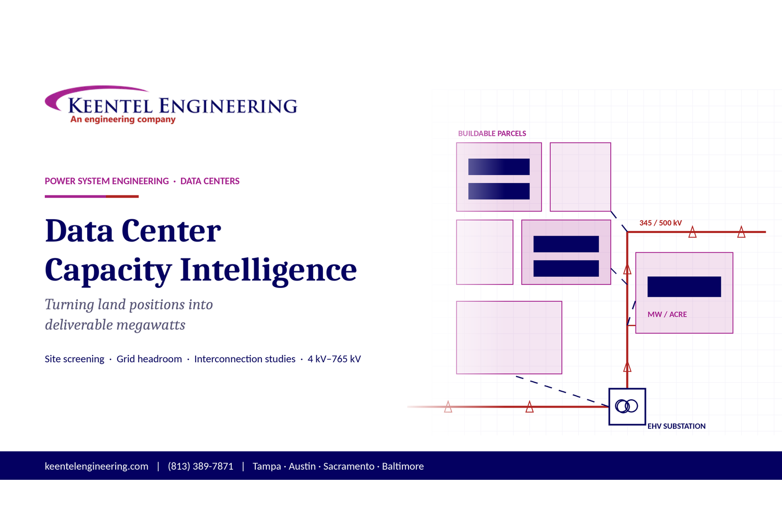
Plan data center capacity with land screening, MW-per-acre estimates, grid power availability and interconnection feasibility studies from Keentel Engineering.
By SANDIP R PATEL
•
October 11, 2026
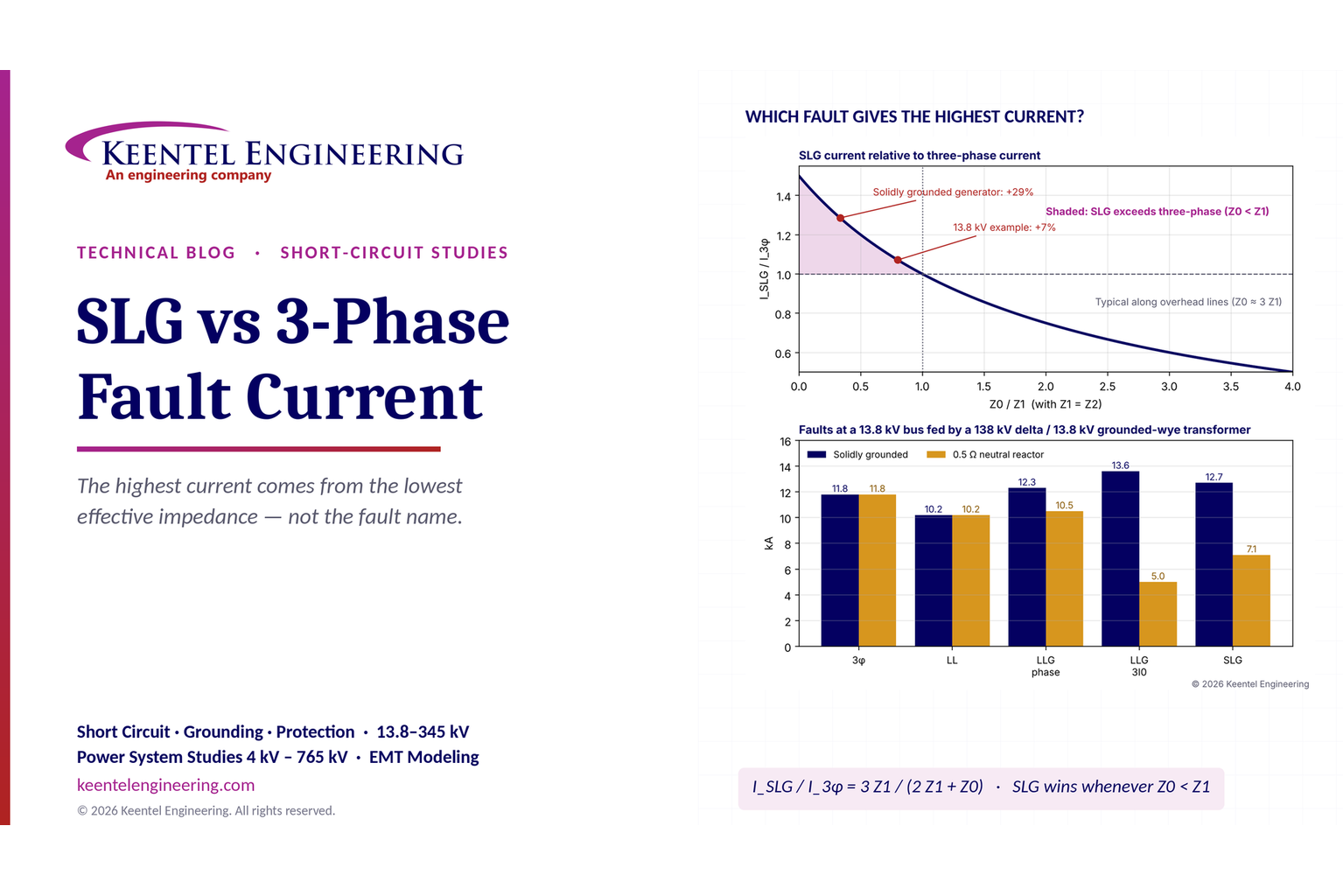
Learn which fault produces the highest current at a bus, why SLG faults can exceed three-phase faults, and how symmetrical components determine fault duty.
By SANDIP R PATEL
•
October 11, 2026
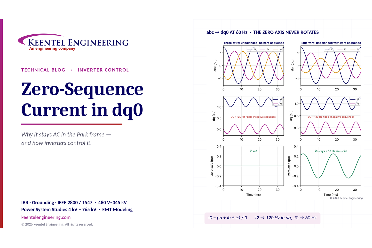
Learn why zero-sequence current pulsates in the dq0 frame, how Park's transformation works, and how inverter controls handle unbalance and ground faults.
By SANDIP R PATEL
•
October 11, 2026
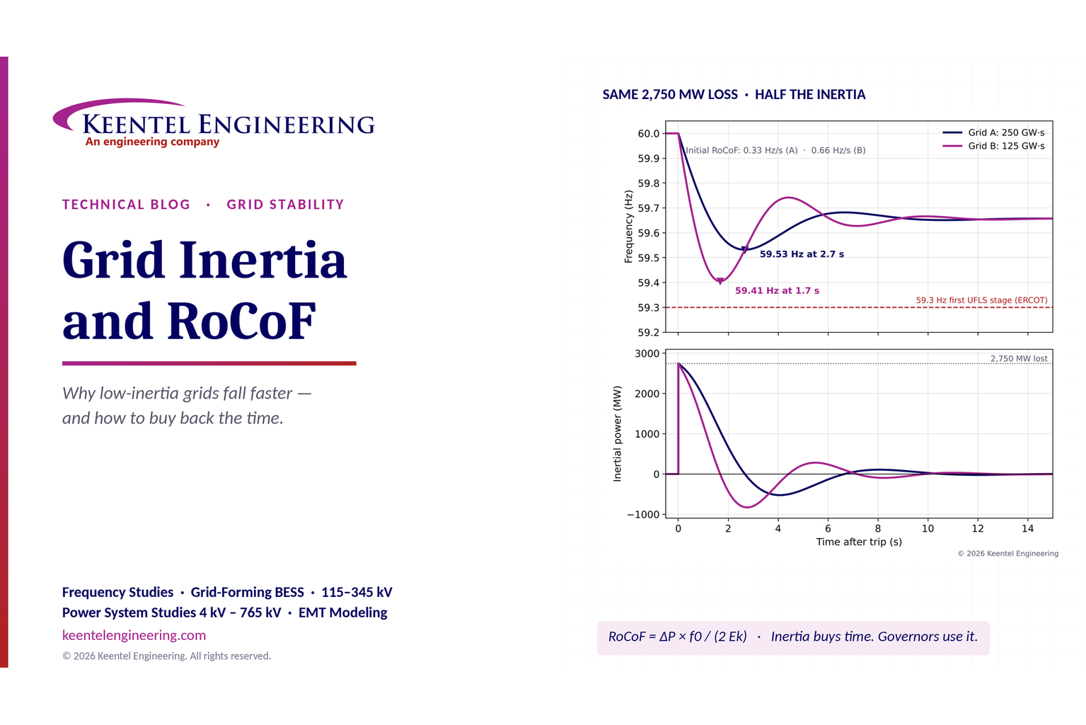
Explore grid inertia, RoCoF and frequency response, with swing equation calculations, frequency nadir analysis and US power system simulation examples.
By SANDIP R PATEL
•
October 11, 2026
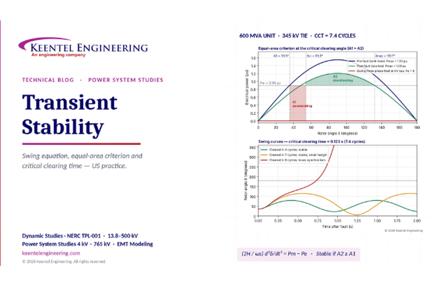
Learn transient stability analysis, swing equation, equal-area criterion and critical clearing time with a 345 kV worked example and NERC TPL-001 guidance.
By SANDIP R PATEL
•
October 11, 2026
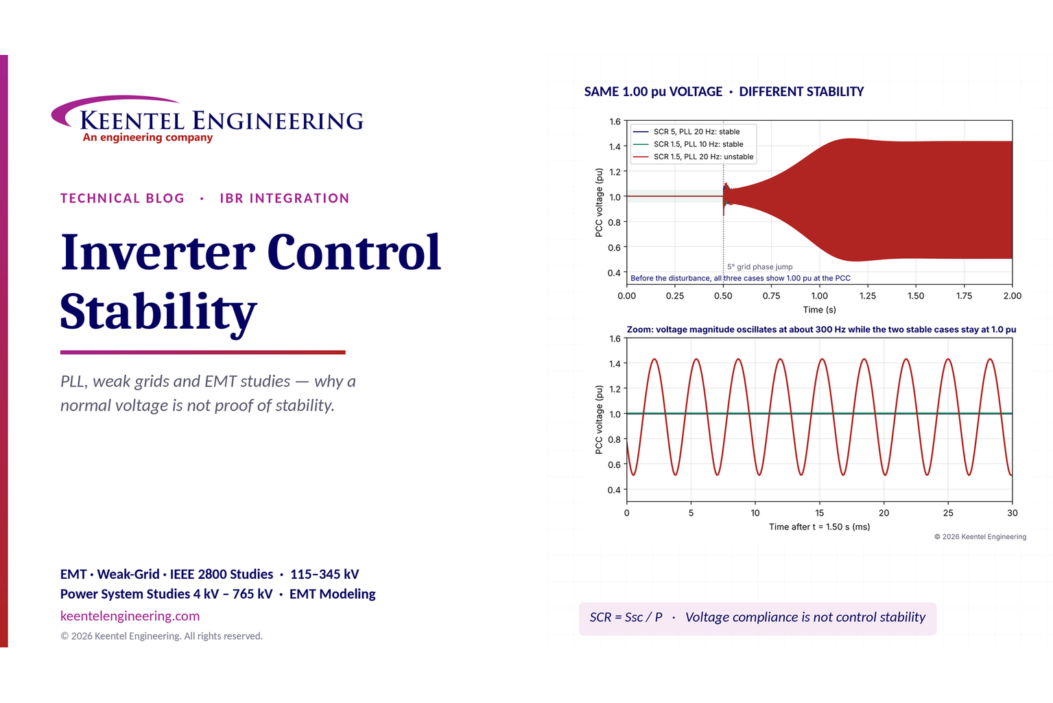
Learn why inverter controls become unstable in weak grids, how PLL bandwidth and SCR affect stability, and how PSCAD EMT studies identify and mitigate oscillations.
By SANDIP R PATEL
•
October 11, 2026
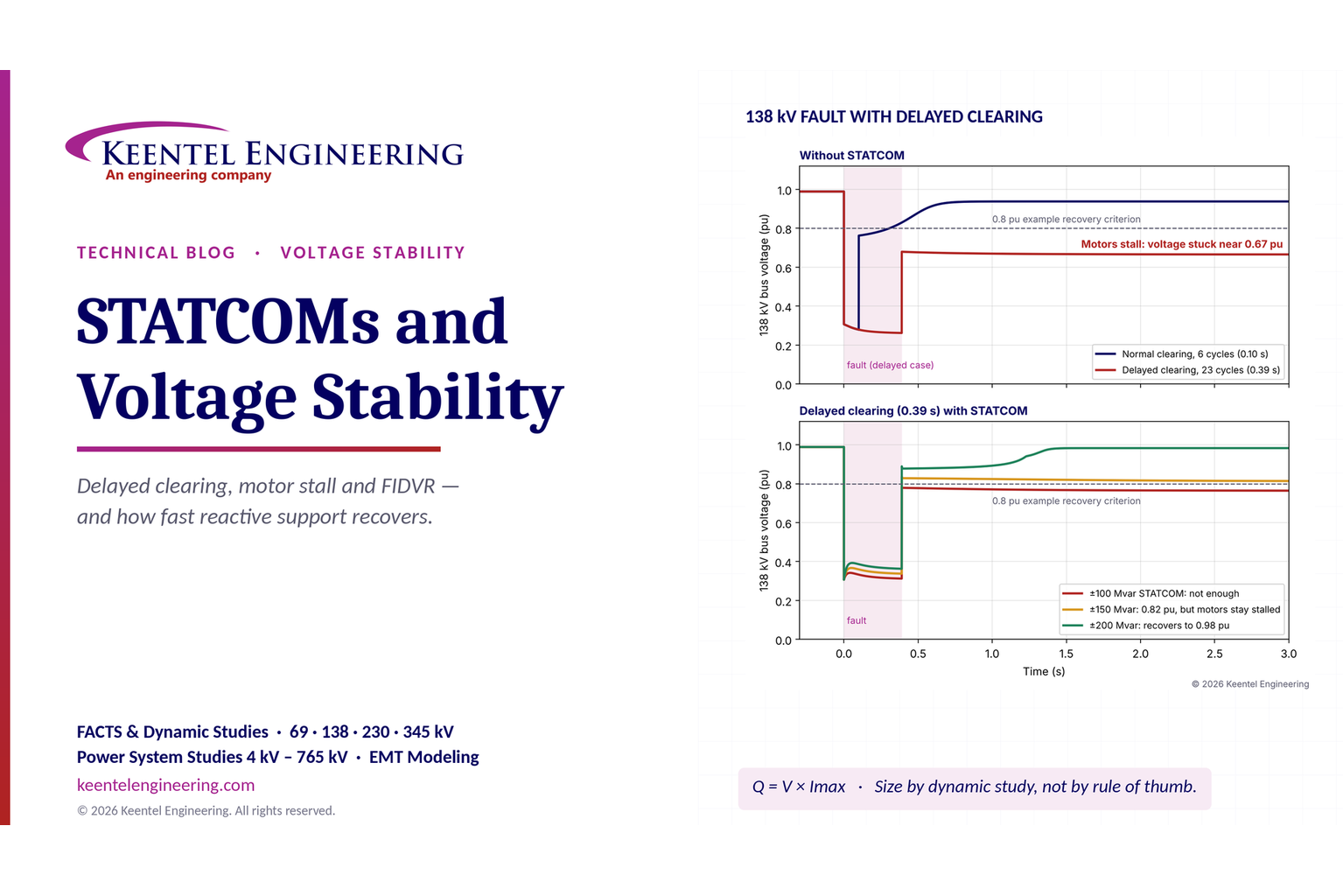
Learn how STATCOMs improve voltage stability and prevent FIDVR. Explore reactive power sizing, delayed fault clearing, NERC criteria and 138 kV simulation results.
By SANDIP R PATEL
•
October 10, 2026
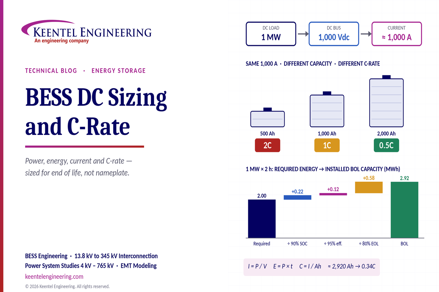
Learn BESS DC sizing with power, energy, current and C-rate calculations, battery losses, degradation and a 100 MW/400 MWh utility-scale example.
By SANDIP R PATEL
•
October 10, 2026
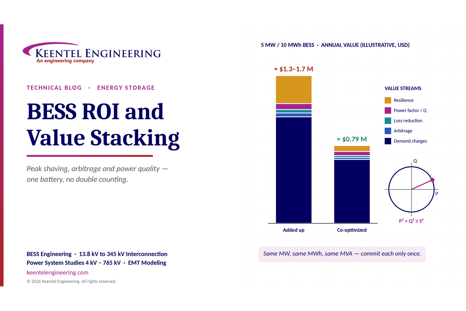
Learn how BESS ROI is calculated using peak shaving, energy arbitrage, power quality and battery storage economics, with a practical 5 MW/10 MWh example.