Part A — Wind Turbine Power Curve Analysis at a Glance
A wind turbine is paid for the energy it delivers, and the power curve is the contract that says how much energy it should deliver. Every utility-scale turbine in the United States is sold with a warranted (or "reference") power curve: a table of expected electrical output at each hub-height wind speed, normalized to a reference air density. Power curve analysis compares what a turbine actually produces with what that curve says it should produce, and turns the difference into answers that matter to an owner:
- Is the turbine really underperforming, or is the measurement wrong?
- If it is underperforming, by how much energy and how much revenue per year — not just by how many kilowatts at one wind speed?
- What is the cause: aerodynamics, control, drivetrain, converter, curtailment, sensors or the site itself?
- What is the fix worth, and how will we prove the fix worked?
The headline formula is simple. At a given wind-speed bin, power curve deviation is

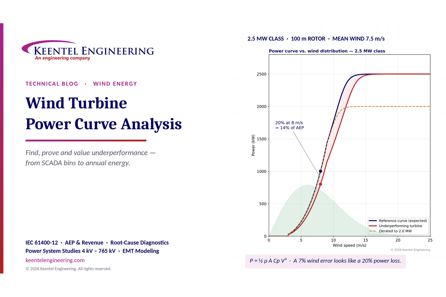
A turbine expected to make 1,000 kW at 8 m/s that makes 800 kW shows a 20% deviation in that bin. That arithmetic is correct. What follows from it usually is not. A 20% gap at one wind speed is not a 20% loss of annual energy or revenue, a 20% gap in power can be produced by only a 7% error in measured wind speed, and a deficit that persists at rated wind speed points to completely different causes than a deficit below rated. Getting from a single-bin deviation to a defensible energy-loss figure and a root cause is an engineering discipline, and that discipline is the subject of this guide.
The turbine in this guide
Keentel Engineering uses an illustrative 2.5 MW-class turbine throughout this guide, typical of the large US land-based fleet installed over the last decade. The turbines sit in a 150 MW wind plant with 34.5 kV collector circuits and a 34.5/230 kV main power transformer.
| Item | Value |
|---|---|
| Rated power | 2,500 kW (variable-speed, pitch-regulated) |
| Rotor diameter / swept area | 100 m / 7,854 m² |
| Cut-in, rated, cut-out wind speed | 3 m/s, about 13–14 m/s (flat plateau from about 14 m/s), 25 m/s |
| Reference air density | 1.225 kg/m³ (sea level, 15 °C) |
| Expected output at 8 m/s | 1,003 kW (electrical power coefficient Cp ≈ 0.41) |
| Site wind regime | Rayleigh distribution (Weibull k = 2), mean hub-height wind speed 7.5 m/s |
| Reference gross AEP | 8,522 MWh/yr per turbine (gross capacity factor 38.9%) |
| Plant | 60 turbines, 150 MW, 34.5 kV collectors, 230 kV point of interconnection |
What Keentel's model shows
Keentel modeled the reference curve at 0.5 m/s bins, weighted it with the site wind distribution, and compared several "underperformance" cases that all start from the same observation — output below the curve.
| Case | Deviation at 8 m/s | Annual energy loss | What it really means |
|---|---|---|---|
| Uniform 20% shortfall at every wind speed, including rated | 20.0% | 20.0% | Only possible if the turbine is also capped below rated — a derate or converter limit, not just aerodynamics |
| 20% loss of aerodynamic efficiency (Cp × 0.80) — pitch offset plus heavy erosion | 20.0% | 14.3%(1,221 MWh/yr) | The turbine still reaches 2,500 kW, only later; rated-wind hours are unaffected |
| Derate to 2,000 kW, aerodynamics healthy | 0.0% | 8.7% | Invisible at 8 m/s; shows only on the plateau |
| Healthy turbine, nacelle anemometer over-reads by 7.2% | 19.1% (apparent) | 0% | A measurement error that looks like a 20% performance problem |
| Yaw misalignment 6° (cos² to cos³ model) | 1.1–1.6% | 0.7–1.1% | Small per turbine, large across a fleet |
| Leading-edge erosion (Cp − 3%) | 3.0% | 2.0% | Typical of moderate erosion on a 7–10-year-old blade set |
| Static pitch offset (Cp − 5%) | 5.0% | 3.3% | Common after blade or pitch-bearing work |
| Drivetrain or generator efficiency − 1.5% | 1.5% | 1.5% | Uniform below and above rated only if the converter has no headroom |

Figure 1. Keentel's power curve model for a 2.5 MW-class turbine. Top: reference curve, a turbine with a 20% loss of power coefficient, and a healthy turbine seen through an anemometer that over-reads by 7.2%, with the site wind-speed distribution shaded. Bottom: lost energy by wind-speed bin — the 20% bin deviation becomes a 14.3% loss of annual energy because the turbine still reaches rated power.
Five lessons
- Measure energy, not one point. A deviation at one bin must be weighted by how many hours the site spends in that bin. In Keentel's model the 8 m/s bin accounts for only about 390 hours a year.
- Suspect the wind measurement first. Power varies with the cube of wind speed. A nacelle anemometer, nacelle transfer function or air-density error of a few percent produces a power "deficit" several times larger.
- Where the gap sits tells you what broke. A gap only below rated is aerodynamic or control-related (pitch, yaw, blade condition). A lower plateau is a derate, a converter or generator limit, or curtailment. A gap only near cut-in suggests drivetrain losses, start-up logic or parasitic load.
- Filter before you conclude. Curtailment, derates, faults, icing, low air density and turbulence must be removed or normalized before any deviation is credible.
- Turn the finding into dollars and a fix. A 14% energy loss on one 2.5 MW turbine is roughly 1,200 MWh and $70,000 a year at an illustrative $60/MWh combined energy and tax-credit value. That justifies an inspection campaign; a 1% loss on a 60-turbine fleet justifies a yaw-calibration program.
Engineering review of common statements about power curves
| Common statement | Keentel's check |
|---|---|
| "A power curve is the relationship between wind speed and electrical power output." | Correct, with qualifications: it is defined at hub height, at a reference air density (usually 1.225 kg/m³), for stated turbulence and shear conditions, and as 10-minute averages grouped into 0.5 m/s bins. Without those qualifiers two curves cannot be compared. |
| Reference curve showing output from about 1 m/s and still rising past 1,200 kW at 16 m/s | Not realistic for a utility-scale turbine. Output starts at cut-in (about 3 m/s), rises steeply in Region 2, and flattens to a constant rated plateau from about 11–14 m/s under pitch control until cut-out (about 20–25 m/s). A machine making 1,000 kW at 8 m/s is a 2–2.5 MW-class turbine with a 90–110 m rotor. |
| "Deviation = [(Reference − Actual) / Reference] × 100; 1,000 kW vs 800 kW at 8 m/s = 20% underperformance." | The arithmetic is right for that bin, provided both values are density-normalized, filtered and binned the same way. It describes one bin, not the turbine. |
| "That is 20% of potential energy — and revenue — lost." | Usually wrong. Energy loss is the deviation weighted by the wind distribution across all bins. In Keentel's model a 20% aerodynamic loss at 8 m/s is a 14.3% energy loss. Revenue also depends on when the energy is lost (prices, curtailment hours) and on tax-credit eligibility. |
| "Pitch faults, yaw misalignment, blade contamination, gearbox and generator issues, derating and sensor errors cause underperformance." | Correct list, but incomplete and unranked. Add air density, turbulence intensity and wind shear (site effects, not faults), wake losses, converter and auxiliary-power limits, control software and parameter changes, and icing. Each cause has a distinct signature on the power curve. |
| "Turbine derating is intentional limitation due to grid or environmental constraints." | Correct. Derates and curtailments are not performance faults and must be filtered out using controller status codes and dispatch records, otherwise they will be misreported as underperformance. |
| "Sensor error means inaccurate anemometer or power readings." | Correct and under-weighted. Because power depends on V³, wind-speed error is the single most common cause of apparent underperformance in nacelle-based analysis. |
Part B — Power Curve Analysis in Technical Depth: Identifying and Diagnosing Underperforming Wind Turbines
1. Why power curve analysis matters to US wind owners
The US land-based wind fleet now exceeds 150 GW, and a large share of it is entering its second decade of operation. Turbines installed between 2008 and 2016 are coming off original manufacturer warranties, blades are showing leading-edge erosion, pitch and yaw systems have accumulated millions of cycles, and many plants are being repowered or re-contracted. At the same time, revenue per MWh has become more sensitive: merchant and hedge settlements depend on when energy is produced, production tax credit (PTC) value is tied to metered energy, and power purchase agreements often carry availability or output guarantees.
In that environment, a few percent of energy matters. On a 150 MW plant with a 38% net capacity factor, 1% of annual energy is about 5,000 MWh. At an illustrative combined value of $60/MWh, that is roughly $300,000 a year — every year, for the remaining life of the plant. Power curve analysis is how owners find that 1%, prove where it went, and decide whether it is worth recovering.
It is also how owners avoid chasing ghosts. Much of the "underperformance" flagged by simple SCADA dashboards is not real. It comes from wind-speed measurement error, from curtailment and derates that were not filtered, or from site conditions (air density, turbulence, shear) that the reference curve does not represent. A disciplined method separates real performance loss from measurement and site artifacts before money is spent on cranes, blade repairs or warranty disputes.
2. The physics behind the power curve
2.1 Power in the wind
The kinetic power in the wind passing through a rotor of swept area A is

where ρ is air density (kg/m³), A is the rotor swept area (m²) and V is the free-stream wind speed at hub height (m/s). A turbine converts a fraction of that power into electricity, described by the power coefficient Cp:

The electrical power coefficient includes the aerodynamic efficiency of the rotor and the losses in the drivetrain, generator and converter. Cp depends on the tip-speed ratio λ and the blade pitch angle β:

where ω is rotor speed (rad/s) and R is the rotor radius (m).
Worked example 1 — the 8 m/s point. For Keentel's 2.5 MW-class turbine (100 m rotor, A = 7,854 m²) at 8 m/s and sea-level density:

The reference curve gives 1,003 kW at 8 m/s, so the electrical power coefficient is about 1,003 / 2,463 = 0.41. That is a realistic value for a modern turbine: aerodynamic Cp of about 0.46–0.48 multiplied by a drivetrain-and-converter efficiency of about 0.88–0.92 at part load.
2.2 The Betz limit
No open rotor can extract more than 16/27 of the power in the wind:

At 8 m/s, the Betz limit for this rotor is about 1,460 kW. Any SCADA record that implies an electrical Cp above about 0.5 is a red flag for wind-speed under-reading, not for an exceptional turbine. Keentel uses the implied Cp as an early data-quality screen.
2.3 The four regions of a real power curve
A utility-scale, variable-speed, pitch-regulated turbine operates in four regions:
| Region | Wind speed (typical) | Control objective | Power behavior |
|---|---|---|---|
| Region 1 | Below cut-in (about 3 m/s) | Turbine idles or yaws; no generation | Zero; small auxiliary consumption |
| Region 2 | Cut-in to about 9–10 m/s | Maximize Cp: hold optimal tip-speed ratio by varying rotor speed (generator torque control), pitch at fine angle | Rises roughly with V³ |
| Region 2.5 (transition) | About 10–14 m/s | Rotor reaches maximum speed; torque rises to rated | Curve bends toward rated |
| Region 3 | Rated to cut-out (about 14–25 m/s) | Hold rated power by pitching blades to feather | Flat plateau at rated power |
Above cut-out (typically 20–25 m/s for land-based turbines, with some models using high-wind ride-through ramps), the turbine pitches to feather and stops or reduces output to protect the structure.
This structure matters for diagnosis. A turbine that is aerodynamically degraded still reaches rated power — only at a higher wind speed — because the pitch controller simply holds the blades at a finer angle to make up the difference. A turbine whose plateau is below rated has a limit, not an efficiency problem: a derate, a converter or generator constraint, a temperature limit or a curtailment set point.
2.4 Why realistic curves matter
Simplified graphics often show a reference curve that starts producing power almost from zero wind speed and keeps rising past 1,200 kW at 16 m/s. Real curves look different: essentially zero output below 3 m/s, a steep rise between 5 and 11 m/s, and a flat top. Using an unrealistic reference curve in analysis guarantees false conclusions, because deviations will appear where none exist (high winds) and disappear where they matter (Region 2).
Rule of thumb. A turbine making about 1,000 kW at 8 m/s is a 2–2.5 MW-class machine with a 90–110 m rotor. If the analysis claims that turbine has a 1,200 kW rating, either the curve or the turbine data are wrong.
2.5 The cubic sensitivity — the most important equation in this guide
Because power varies with V³ in Region 2, a small wind-speed error becomes a large power error:

More exactly, if measured wind speed is too high by a factor k, a healthy turbine appears to produce

Worked example 2 — a 20% "loss" from a 7% wind error. Solve for the wind-speed error that produces a 20% apparent deficit:

An anemometer or nacelle transfer function that over-reads by 7–8% makes a perfectly healthy turbine look 20% short in Region 2. Keentel's model (Figure 1) shows a 7.2% over-read producing a 19% apparent deficit at 8 m/s. In the transition region the apparent deficit is smaller, and on the rated plateau it disappears — which is itself a diagnostic clue.
Typical sources of wind-speed error of this size include a nacelle anemometer that has been replaced with a different model, a changed or incorrect nacelle transfer function after a software update, a damaged or iced cup or ultrasonic sensor, a misaligned sensor boom, and blade-wake effects that change after blade modifications such as vortex generators.
3. The power curve as a contract: reference, warranted and measured curves
Three different curves are often called "the power curve." Mixing them up is the most common source of disputes.
| Curve | Who defines it | Basis | Use |
|---|---|---|---|
| Reference (published) curve | Turbine manufacturer | Design calculation and type testing at reference density and standard turbulence | Energy yield assessment, project financing |
| Warranted (contractual) curve | Turbine supply agreement | Usually the reference curve at a stated density, with a tolerance (for example 95% of AEP) and specified test conditions | Warranty claims and liquidated damages |
| Measured curve | Owner or independent tester | Field measurement to a standard procedure, or SCADA-based operational analysis | Performance verification, diagnosis, claims |
Turbine supply agreements typically warrant a power curve indirectly: the warranted quantity is the annual energy production (AEP) calculated from the measured power curve and a reference wind distribution (often Rayleigh with a stated mean), compared against AEP calculated from the warranted curve. A tolerance band — often in the range of 95% of warranted AEP — and the measurement uncertainty determine whether the test passes. Owners should read three clauses closely: the reference air density and the density-correction method, the allowed site conditions (turbulence, shear, terrain), and how measurement uncertainty is treated in the pass/fail calculation.
4. Measuring a power curve correctly
4.1 Standards used in US practice
Power performance testing in the United States follows the international standards of the IEC 61400 series, which are referenced in virtually every US turbine supply agreement. There is no separate IEEE or ANSI power-performance test standard for wind turbines; US practice adopts the IEC methods directly.
| Standard | Scope | Typical use |
|---|---|---|
| IEC 61400-12-1 (Ed. 3, 2022) | Power performance of electricity-producing wind turbines using a met mast or remote sensing (lidar) upwind of the turbine | Contractual power curve verification; the reference method |
| IEC 61400-12-2 (Ed. 2, 2022) | Power performance using nacelle anemometry with a nacelle transfer function (NTF) | Fleet testing where masts are impractical |
| IEC 61400-12-3 | Measurement-based site calibration | Complex terrain, before 12-1 testing |
| IEC 61400-50-2 and 50-3 | Ground-based and nacelle-mounted lidar | Remote-sensing wind measurement |
| IEC 61400-26-1 and 26-2 | Time-based and production-based availability | Availability definitions for contracts and KPIs |
| IEC 61400-21-1 | Electrical characteristics measurement | Power quality and grid-related tests |
4.2 The method in brief
The core of IEC 61400-12-1 is straightforward:
- Measure hub-height wind speed (ideally rotor-equivalent wind speed), wind direction, air temperature, pressure and humidity, and turbine electrical power at the low-voltage terminals or the turbine transformer.
- Sample at 1 Hz or faster and compute 10-minute averages and standard deviations.
- Select data from a valid measurement sector — wind directions free of wakes from other turbines and obstacles.
- Exclude periods when the turbine is not in normal operation (faults, manual stops, curtailment, derates, icing) and periods with equipment failures.
- Normalize wind speed to reference air density.
- Bin the data in 0.5 m/s wind-speed bins and average power within each bin (method of bins).
- Check completeness: at least 180 hours of valid data overall, at least 30 minutes in each bin, and a wind-speed range from 1 m/s below cut-in to 1.5 times the wind speed at 85% of rated power.
- Calculate AEP with Rayleigh distributions at standard mean wind speeds (4–11 m/s) and report uncertainty.
The measured power in bin i is

and the normalized wind speed is the bin average of the density-normalized 10-minute wind speeds.
4.3 Air-density normalization
For a pitch-regulated turbine with active power control, the standard normalizes wind speed rather than power:

with ρ0 the reference density (usually 1.225 kg/m³). The 10-minute density comes from measured temperature and pressure (and, in the current edition, humidity):

where B is barometric pressure (Pa), T is absolute temperature (K) and R0 is the gas constant of dry air, 287.05 J/(kg·K).
Worked example 3 — a high-plains site. A wind plant at 1,200 m elevation sees an annual-average temperature of about 15 °C. Standard-atmosphere pressure at that elevation is about 87.7 kPa, so

In summer at 30 °C it falls to about 1.008 kg/m³. If an analyst plots raw SCADA wind speed against power and compares the result with the sea-level reference curve, the turbine appears to make 13% less power in Region 2 — at 8 m/s, about 869 kW instead of 1,003 kW — with no fault at all. Normalizing correctly moves a measured 8.0 m/s to 7.63 m/s, where the reference curve predicts 868 kW. The "deficit" disappears.
Air density is the first correction Keentel applies, and it is the most frequently omitted one in in-house dashboards serving plants in the Great Plains, Mountain West and Texas Panhandle.
4.4 Turbulence and wind shear
The power curve is a function of more than mean wind speed. Two site effects change it measurably:
Turbulence intensity (TI) is the ratio of the 10-minute standard deviation of wind speed to the mean:

Because power is a curved (non-linear) function of wind speed, averaging over turbulent fluctuations biases the 10-minute power. High turbulence raises apparent power near cut-in (the convex part of the curve) and lowers it near rated (the concave knee). A turbine at a site with 18% TI will show a rounder knee and a lower apparent output at 11–13 m/s than the same turbine tested at 8–10% TI. IEC 61400-12-1 Annex M gives a turbulence normalization method that removes this effect by building a zero-turbulence curve and re-simulating it at the reference TI.
Wind shear describes how wind speed changes with height, often approximated by a power law:

A hub-height measurement does not represent the kinetic energy flux across a 100 m rotor when shear is strong (for example α of 0.25–0.35 in stable night-time conditions on the Great Plains) or when the profile has a low-level jet. The rotor-equivalent wind speed corrects for this:

where Vi is the wind speed at the height of rotor segment i, measured by lidar or a tall mast. Without it, night-time and daytime power curves at the same hub-height wind speed can differ by several percent, and a turbine can appear to underperform only at night.
4.5 Measurement uncertainty
Every measured power curve carries uncertainty, and contractual tests weigh it explicitly. The standard splits uncertainty into:
- Category A (statistical): the scatter of power within each bin.
- Category B (systematic): instrument calibration and mounting, power transducer accuracy, air-density measurement, site calibration, terrain and the method itself.
The Category A uncertainty in bin i is

Worked example 4 — bin uncertainty at 8 m/s. With 40 valid 10-minute records in the 8 m/s bin and a standard deviation of 120 kW, the statistical uncertainty is 120/√40 ≈ 19 kW, or about 1.9%. The Category B contribution from wind speed dominates: a 2% wind-speed uncertainty at 8 m/s, combined with a curve slope of about 380 kW per m/s, gives

That is about 6% of bin power. Combining the components, the AEP uncertainty for a well-executed mast-based test is typically 4–7%; nacelle-anemometry tests are higher. A claimed 3% underperformance measured with 6% uncertainty is not a finding; it is a hypothesis.
5. From bin deviation to energy and revenue
5.1 Annual energy production by the method of bins
AEP is the power curve weighted by the hours spent at each wind speed:

where Nh = 8,760 hours and F(V) is the cumulative wind-speed distribution. For a Weibull distribution with shape k and scale c,

The Rayleigh distribution is the special case k = 2, and its scale is set by the mean wind speed:

5.2 Worked example 5 — the 20% deviation turned into energy
Keentel's model compares the reference curve with a turbine that has lost 20% of its power coefficient — the deviation shown at 8 m/s in the example that opened this guide. The table uses 1 m/s bins for readability (the figure and the headline numbers use 0.5 m/s bins).
| Wind speed (m/s) | Hours per year | Reference power (kW) | Degraded power (kW) | Reference energy (MWh) | Energy lost (MWh) |
|---|---|---|---|---|---|
| 3 | 645 | 30 | 24 | 19 | 4 |
| 4 | 780 | 102 | 82 | 80 | 16 |
| 5 | 860 | 226 | 181 | 195 | 39 |
| 6 | 886 | 411 | 329 | 364 | 73 |
| 7 | 862 | 666 | 533 | 574 | 115 |
| 8 | 800 | 1,003 | 802 | 802 | 160 |
| 9 | 710 | 1,433 | 1,147 | 1,017 | 203 |
| 10 | 605 | 1,764 | 1,415 | 1,068 | 211 |
| 11 | 497 | 2,101 | 1,709 | 1,044 | 194 |
| 12 | 394 | 2,354 | 2,014 | 926 | 134 |
| 13 | 301 | 2,462 | 2,277 | 741 | 56 |
| 14 | 223 | 2,491 | 2,426 | 554 | 14 |
| 15–25 | 464 | about 2,500 | about 2,500 | 1,161 | 4 |
| Total | 8,760(incl. below cut-in) | 8,545 | 1,223 (14.3%) |
Three conclusions follow:
- The loss is 14.3% of AEP, not 20%. About 40% of this turbine's energy is produced at 11.5 m/s and above, where the pitch controller compensates for lost aerodynamic efficiency.
- The biggest losses are at 9–11 m/s, not at 8 m/s. The 8 m/s bin is not the most important one; the transition region is, because it combines high power with many hours.
- Site wind regime changes the answer. At a lower-wind site (mean 6.5 m/s), the same degradation costs a larger share of AEP because less energy comes from the rated plateau. At a higher-wind site (mean 8.5 m/s) it costs less.
5.3 Worked example 6 — revenue
For one turbine, 1,223 MWh/yr at an illustrative $60/MWh combined value (power purchase agreement price plus production tax credit) is about $73,000 per year. If the same problem affected all 60 turbines in a 150 MW plant, the loss would be about 73,000 MWh and $4.4 million per year.
The value used should reflect the project. The PTC applies to metered energy for the first ten years of a qualifying facility's operation, is inflation-adjusted (on the order of 3 ¢/kWh in recent years for projects meeting prevailing-wage and apprenticeship requirements), and its availability for new projects was narrowed by federal legislation in 2025. Owners should confirm their credit status with tax counsel. Merchant energy should be valued at the realized price in the hours it was lost — energy lost on windy nights in a congested zone may be worth far less than the average price.
5.4 Worked example 7 — the derate that hides at 8 m/s
A turbine derated to 2,000 kW shows zero deviation at 8 m/s, yet loses 8.7% of AEP (about 740 MWh/yr) because every hour above about 10.5 m/s is capped. A bin-deviation dashboard keyed to Region 2 will never find it. Owners should track the plateau separately and reconcile any derate with its authorization (grid instruction, environmental curtailment, warranty-mandated derate or a forgotten maintenance setting).
6. Operational power curve analysis with SCADA data
Contractual tests are expensive and infrequent. Day-to-day performance monitoring uses the turbine's own SCADA data: 10-minute averages of nacelle wind speed, power, rotor and generator speed, pitch angle, yaw position, nacelle direction, temperatures and status codes. Done well, SCADA-based analysis detects most real problems within weeks. Done poorly, it generates false alarms that erode trust in the whole program.
6.1 The nacelle anemometer problem
The nacelle anemometer sits behind the rotor, in air that the rotor has already slowed and disturbed. Turbine controllers convert that reading to an estimate of free-stream wind speed with a nacelle transfer function (NTF). The NTF depends on the rotor, the blade set, the sensor type and its exact position, and on the controller's operating point. Three practical consequences follow:
- Nacelle wind speed is fine for comparing a turbine with itself over time and with identical neighbors. It is weak evidence for absolute performance against a warranted curve.
- Any change to the sensor, its mounting, the blades (including add-ons such as vortex generators or serrations) or the controller software can shift the NTF and create a step change in apparent performance with no change in real output.
- Ultrasonic sensors and cup anemometers age and fail differently: cups slow down as bearings wear (making the turbine look better), while ultrasonic sensors can drift or suffer offsets from icing, insects or heating faults.
IEC 61400-12-2 describes how to derive and validate an NTF against a met mast or lidar. Keentel recommends that owners keep a record of every sensor replacement, software update and blade modification so that apparent step changes can be explained.
6.2 A defensible SCADA data pipeline
| Step | Purpose | Typical rule |
|---|---|---|
| 1. Time alignment | Align SCADA, met and meter data | Common UTC time base; check clock drift against the 230 kV revenue meter |
| 2. Status filtering | Keep only normal operation | Remove periods with fault, stop, maintenance, curtailment, derate, power-limit, noise-mode, bat or bird curtailment, ice and low-temperature codes |
| 3. Range and stuck-value checks | Remove sensor failures | Flat-lined wind speed, zero power with high wind, negative power above cut-in |
| 4. Physics check | Remove impossible points | Implied electrical Cp above 0.50; power above rated plus tolerance |
| 5. Density normalization | Remove site and seasonal density effect | Vn = V (ρ/ρ0)^(1/3) using site temperature and pressure |
| 6. Sector and wake screening | Remove waked or obstructed directions | Exclude sectors within about 10–20 rotor diameters downwind of neighbors where wakes dominate |
| 7. Outlier removal within bins | Remove residual anomalies | Robust methods (median absolute deviation) rather than fixed percentage cut-offs |
| 8. Binning | Build the curve | 0.5 m/s bins, minimum record count per bin |
| 9. Comparison | Quantify deviation | Against warranted curve, the turbine's own baseline and its peers |
| 10. Energy weighting | Convert deviation into AEP and revenue | Site long-term wind distribution, not a generic Rayleigh |
The order matters. Filtering by status before density normalization avoids normalizing curtailed points; outlier removal after binning avoids discarding legitimate underperformance as noise.
6.3 Residual tracking and control charts
For continuous monitoring, Keentel tracks the energy-weighted residual between expected and measured production:

summed over valid 10-minute records j in each day or week, where the expected power comes from the turbine's own validated baseline curve rather than the generic reference. A cumulative-sum (CUSUM) chart then detects small persistent shifts that a daily plot hides:

with an alarm when St exceeds a threshold h. Choosing k0 at about half the shift worth detecting (for example 0.5% for a 1% shift) and h at four to five standard deviations of the daily residual gives a practical balance between early detection and false alarms. A 2% step change in Region 2 performance on a turbine with typical SCADA scatter is usually detected in two to four weeks.
6.4 Fleet peer comparison
Turbines of the same model, in similar positions in the same plant, should perform within a narrow band. A peer comparison computes each turbine's production ratio against the median of its neighbors during the same hours:

A turbine that sits 3–5% below its peers for months, with no difference in wake exposure or terrain, has a real problem even if its nacelle-based curve looks close to the warranted curve. Peer comparison is also the best defense against systematic nacelle wind-speed errors, because the comparison uses energy rather than wind speed.
7. Causes of underperformance and their signatures
The single most useful skill in power curve analysis is reading where and how the measured curve departs from the reference. The table below summarizes the signatures Keentel uses as a first pass.
| Cause | Region 2 (cut-in to about 10 m/s) | Transition (about 10–14 m/s) | Rated plateau | Other evidence |
|---|---|---|---|---|
| Pitch offset (static) on all blades | Lower, proportionally | Reaches rated later | Normal | Pitch angle vs wind speed differs from fleet; Cp vs λ shifted |
| Pitch imbalance (one blade) | Slightly lower | Slightly lower | Normal | Rotor imbalance, 1P vibration, tower loads |
| Yaw misalignment | Lower, by about cos² to cos³ of the error | Lower | Normal (if enough wind) | Nacelle-vs-wind direction offset; lidar or spinner anemometer |
| Leading-edge erosion, dirt, insects | Lower (1–5% AEP) | Reaches rated later | Normal | Worse after dry, buggy summers; visible on drone inspection |
| Icing | Strongly lower, erratic | Lower | Possibly lower | Low temperature and high humidity; ice-detection codes |
| Gearbox or generator efficiency loss | Lower by a near-constant kW or % | Lower | Lower only if converter limits by mechanical input | Rising oil or winding temperatures |
| Converter or electrical limit | Normal | Flattened early | Below rated | Temperature or current limit codes |
| Derate or curtailment | Normal | Flattened early | Below rated, at a set point | Controller limit codes; dispatch or environmental instruction |
| Anemometer or NTF error | Shifted left or right (looks better or worse) | Shifted | Normal | Step change after sensor or software work; peers disagree |
| Low air density (not normalized) | Lower by about ρ/ρ0 | Rated reached later | Normal | Seasonal pattern; elevation |
| High turbulence | Higher near cut-in | Lower and rounder knee | Normal | TI from 10-minute standard deviation |
| Wake losses | Lower in waked sectors only | Lower | Normal | Direction-dependent; matches layout |
| Start-up and cut-in logic | Lower or missing near cut-in | Normal | Normal | Frequent start-stop cycling |
| Auxiliary load (heaters, cooling) | Lower net near cut-in | Normal | Slightly lower | Seasonal; consumption visible at idle |
7.1 Pitch system faults and offsets
The pitch system sets the blade angle. In Region 2 the blades should sit at the "fine" pitch angle that maximizes Cp. A static offset of even 1–2° — from a mis-set encoder after a blade bearing replacement, a wrong parameter, or a blade mounted with an incorrect zero mark — reduces Cp across the whole of Region 2. Keentel's model shows that a 5% Cp loss, which a 1.5–2° offset can produce on some rotors, costs about 3.3% of AEP.
Diagnostics include plotting pitch angle against wind speed for each turbine and its peers (offsets show as a shifted curve), calculating Cp against tip-speed ratio from SCADA data, and photographic or laser blade-angle measurement during a maintenance stop. Single-blade misalignment is better detected by rotor imbalance and 1P vibration than by the power curve.
7.2 Yaw misalignment
When the rotor is not facing the wind, the component of wind speed perpendicular to the rotor falls by the cosine of the yaw error γ. Theory suggests power falls with cos³γ; field data commonly show an exponent closer to 2. Keentel uses a range:

Worked example 8 — a 6° offset. cos²(6°) = 0.989 and cos³(6°) = 0.984, so power in Region 2 falls by 1.1–1.6%. Weighted over the wind distribution — including the rated plateau where yaw error costs little — the AEP loss in Keentel's model is 0.7–1.1%. Across a 60-turbine plant, that is 3,600–5,600 MWh a year, which pays for a yaw-calibration campaign many times over.
Static yaw offsets usually come from wind-vane mounting errors, a wind vane replaced without recalibration, or an incorrect north or vane offset parameter. Nacelle-mounted lidar or spinner anemometry over a few weeks can measure the offset directly. A SCADA-only method fits power against the vane-reported relative wind direction and finds the angle at which power peaks.
7.3 Blade contamination, erosion and icing
Leading-edge erosion roughens the most aerodynamically sensitive part of the blade, triggering early transition to turbulent flow and reducing lift-to-drag ratio. Published field and wind-tunnel studies put the AEP loss from moderate to severe erosion in the range of about 1% to 5%, with higher values in extreme cases. Erosion is progressive and depends on rain, hail, dust and tip speed; tip speeds above about 80 m/s accelerate it. Insect build-up and dirt produce smaller, often seasonal losses that rain can partly wash away.
Icing is different in kind: it can reduce output dramatically, change blade mass and loads, and create ice-throw hazards. Ice-affected periods should be flagged and excluded from performance baselines but tracked separately as an energy-loss category, because ice protection systems and operating strategies have measurable value at cold-climate US sites.
Diagnostics include drone or crawler blade inspections graded on a consistent erosion scale, comparison of the Region 2 curve before and after leading-edge protection repairs, and cold-weather filtering (temperature below about 2 °C with high humidity).
7.4 Gearbox and generator issues
Drivetrain losses reduce the electrical output for a given rotor power. A failing gearbox bearing, high oil viscosity at low temperature or a degraded generator winding typically raises losses by a few percent and raises component temperatures. Because the pitch controller regulates electrical power on the plateau, mechanical losses are usually hidden at rated wind unless they push a component to a thermal limit, at which point the controller derates the turbine.
Signature: a near-constant shortfall of a few tens of kilowatts across Region 2, rising temperatures at the same load, and in advanced cases vibration signatures from condition monitoring. Power curve analysis should be read alongside the condition monitoring system, not instead of it.
7.5 Turbine derating and curtailment
Derates and curtailments are deliberate and are not performance faults. They include:
- Grid curtailment — instructions from the Transmission Operator, Balancing Authority or ISO/RTO for congestion, voltage or reliability, delivered through the plant controller or by economic dispatch.
- Environmental curtailment — bat curtailment at low wind speeds on summer nights, bird detection systems, and noise or shadow-flicker modes.
- Equipment derates — temperature limits, converter limits, manufacturer-mandated derates during a known issue, and derates left in place after maintenance.
The danger is the last category: a derate left in the controller after work, or a manufacturer derate that outlived its purpose. Every derate should map to an authorization, an expected duration and an owner.
Note that NERC ride-through standards (PRC-024-4 for Type 1 and Type 2 wind turbines, and PRC-029-1 for inverter-based Type 3 and Type 4 turbines) govern how turbines behave during grid voltage and frequency disturbances; they are not a cause of steady-state power curve deficits. A turbine tripping during grid disturbances shows up in availability and in event analysis under PRC-030-1, not in the power curve.
7.6 Sensor errors
Sensor error is the most common cause of apparent underperformance and the cheapest to fix. Wind-speed errors are discussed in Section 2.5 and 6.1. Power-measurement errors also matter: a turbine power transducer with a wrong current transformer ratio, a missing phase or a scaling error can misreport power by several percent. Keentel reconciles the sum of turbine SCADA energy against the plant's revenue meter at the 230 kV point of interconnection after accounting for electrical losses (Section 8). A persistent discrepancy larger than expected losses identifies either a power-transducer problem or unaccounted losses.
7.7 Control software and parameter changes
Turbine controllers are updated throughout a turbine's life. A change to the optimal-mode gain, the minimum rotor speed, the pitch schedule, the cut-in logic or the NTF can shift the measured power curve up or down overnight. Owners should require a change record from the operator or manufacturer for every software or parameter update, and Keentel compares the turbine's curve in matched windows before and after each change.
8. Electrical context: from turbine terminals to the point of interconnection
Power curves are defined at the turbine output. Revenue is metered at the point of interconnection (POI). In between, a typical US wind plant has:
- A turbine generator at low voltage (often 690 V) — a doubly-fed induction generator (Type 3) or a full-converter machine (Type 4).
- A pad-mounted or nacelle step-up transformer to 34.5 kV.
- Underground and overhead 34.5 kV collector circuits, each carrying 15–30 MW.
- A collector substation with a 34.5/138 kV, 34.5/230 kV or 34.5/345 kV main power transformer, depending on the interconnection.
- A generator tie line to the utility's POI substation and the revenue meter.
8.1 Electrical losses
Typical full-load electrical losses from turbine terminals to POI are about 2–4% of output, and annual-average losses are lower because losses scale with the square of current. Keentel estimates collector losses feeder by feeder. For a radial feeder with turbines evenly distributed along it, the I²R loss is about one third of the loss that would occur if the full current flowed through the whole feeder:

where I is the feeder current at the substation end and Rφ is the per-phase resistance of the whole feeder.
Worked example 9 — collector losses. A 34.5 kV feeder carries ten 2.5 MW turbines (25 MW) at 0.98 power factor:

With a per-phase feeder resistance of 0.25 Ω, the full-load loss is about 427² × 0.25 ≈ 46 kW, or 0.18% of feeder output. Pad-mounted transformer losses (about 1% at full load, including no-load losses that run continuously) and the main power transformer (about 0.3–0.5%) dominate. Because transformer no-load losses run whenever the transformer is energized, they are a larger share of energy in low-wind months.
Keentel's loss model lets an owner reconcile turbine SCADA energy with POI metered energy month by month. Unexplained gaps above about 0.5–1% justify investigation of power transducers, revenue metering or collector equipment.
8.2 Availability metrics
Power curve performance and availability are different measures, and both are needed. Time-based availability (IEC 61400-26-1) counts the hours a turbine was able to operate. Production-based or energy-based availability (IEC 61400-26-2) compares actual energy with the energy the turbine would have produced had it been available, using the power curve to estimate lost production during downtime:

Energy-based availability is the better commercial measure because an hour lost at 12 m/s is worth far more than an hour lost at 4 m/s. But it depends on a trustworthy power curve — another reason to validate the curve first.
8.3 Links to NERC reliability standards
Power curve and performance analysis touch several NERC obligations for Generator Owners of Bulk Electric System wind plants:
| Standard | Relevance to power curve work |
|---|---|
| MOD-025 | Verification of real and reactive power capability. Capability tests and the plant's real-power limits should agree with turbine and collector limitations identified in performance analysis. |
| MOD-026 and MOD-027 (and the IBR-specific revisions now replacing them) | Verification of dynamic models. Turbine control parameters changed during performance remediation (pitch schedules, power limits, plant controller settings) may change the dynamic model and trigger model updates. |
| MOD-032 | Modeling data submitted to the Planning Coordinator and Transmission Planner; should reflect as-built and as-modified equipment. |
| PRC-028-1 | Disturbance monitoring for inverter-based resources. Its sequence-of-events and turbine fault-code recording is valuable evidence when separating disturbance trips from steady-state underperformance. |
| PRC-029-1 and PRC-024-4 | Ride-through. Disturbance trips are not power curve deficits but do appear as lost energy and availability. |
| PRC-030-1 | Identification and analysis of unexpected changes in IBR output during system events. |
| CIP-003 and related CIP standards | Remote access to turbine SCADA for performance analysis must respect the plant's cyber security controls. |
Small, customer-sited wind turbines fall under NEC Article 694 (Wind Electric Systems), and the turbine itself is typically certified to the small wind turbine standards accepted in the United States. Utility-scale plants under exclusive utility control are generally governed by the National Electrical Safety Code (NESC, ANSI C2) rather than the NEC for their supply-side facilities; owners should confirm which code applies to each part of the plant with the authority having jurisdiction.
9. A practical underperformance investigation workflow
Keentel follows a staged approach that spends effort in proportion to evidence.
| Stage | Question | Methods | Typical duration |
|---|---|---|---|
| 1. Screen | Is any turbine outside its normal band? | Peer production ratios, CUSUM on residuals, plateau check | Continuous |
| 2. Validate data | Is the deviation real? | Status filtering, density normalization, sensor history, revenue-meter reconciliation | 1–2 weeks |
| 3. Locate | Where on the curve is the deviation? | Region 2 vs transition vs plateau; direction and time-of-day splits | 1 week |
| 4. Hypothesize | Which causes fit the signature? | Signature table (Section 7), pitch-vs-wind, Cp vs λ, yaw-power fit | 1 week |
| 5. Confirm | What is physically wrong? | Blade and pitch inspection, nacelle lidar, vane calibration, controller parameter audit, condition monitoring | 2–8 weeks |
| 6. Quantify | What is it worth? | Energy-weighted loss using the long-term site wind distribution; revenue at realized prices | 1 week |
| 7. Fix and verify | Did the fix work? | Matched before/after windows; peer comparison; uncertainty statement | 1–3 months of data |
9.1 Verifying a fix
Before-and-after comparisons are vulnerable to seasonal changes in air density, turbulence and shear. Keentel uses three safeguards: comparing the treated turbine with untreated peers over the same period (a difference-in-differences approach), matching wind direction and turbulence distributions between the two windows, and reporting the improvement with its uncertainty. An improvement of 2% ± 1.5% is real; an improvement of 2% ± 4% is not yet proven.
10. Common misconceptions corrected
| Misconception | Correction |
|---|---|
| A 20% deviation at one wind speed means 20% lost revenue. | Energy loss is the deviation weighted across all wind speeds. In a typical case it is smaller, and revenue depends on when the energy was lost. |
| The reference curve keeps rising with wind speed. | Pitch-regulated turbines hold a flat rated plateau from roughly 12–14 m/s to cut-out. |
| A nacelle-based power curve proves a warranty breach. | Contractual verification requires the test method and site conditions defined in the turbine supply agreement, normally IEC 61400-12-1. Nacelle data supports screening and peer comparison. |
| Lower output at a high-elevation site means the turbine is faulty. | Air density can account for a 10–15% Region 2 shortfall. Normalize first. |
| Derates are not performance problems, so they can be ignored. | Authorized derates are excluded from performance metrics but must be tracked as an energy-loss category; unauthorized or forgotten derates are real losses. |
| Yaw misalignment only matters if it is large. | A 6° offset costs about 1% of AEP; across a fleet that justifies correction. |
| Blades either work or they don't. | Erosion degrades performance progressively; trending detects it before it becomes structural damage. |
11. Key takeaways
- Use a realistic, density-referenced warranted curve and define exactly what you are comparing against.
- Filter status codes and normalize air density before computing any deviation.
- Convert bin deviations to energy using the site's long-term wind distribution, then to revenue at realized prices.
- Read the shape of the deviation: Region 2 problems are aerodynamic or control-related; plateau problems are limits.
- Treat wind-speed measurement as a suspect until proven otherwise — a 7% wind error looks like a 20% power loss.
- Use peer comparison and CUSUM residuals for early detection; reserve contractual tests for claims.
- Verify every fix with matched data and an uncertainty statement.
12. How Keentel Engineering helps
Keentel Engineering supports wind plant owners, investors, asset managers and operators with independent, engineering-grade performance analysis — from the turbine terminals through 34.5 kV collector systems to 138 kV, 230 kV and 345 kV interconnections.
| Service | Keentel scope | Outcome |
|---|---|---|
| Power curve and AEP assessment | SCADA data pipeline, density and turbulence normalization, binned curves, energy-weighted loss and revenue impact | A defensible number for lost energy and its value |
| Underperformance diagnostics | Signature analysis, pitch and yaw analysis, Cp–λ analysis, peer comparison, CUSUM monitoring | Root causes ranked by evidence and value |
| Warranty and contract support | Review of warranted power curve clauses, test planning to IEC 61400-12-1 and 12-2, independent review of test reports | Stronger positions in warranty discussions |
| Electrical loss and metering reconciliation | Collector, transformer and generator tie loss models; revenue-meter versus SCADA reconciliation | Losses explained and metering issues found |
| Repowering and upgrade evaluation | Before/after performance verification of blade upgrades, leading-edge protection, controller updates and repowering | Measured return on upgrade capital |
| Grid and NERC support | MOD-025, MOD-026/027, MOD-032 model and capability work; PRC-028/029/030 data and event analysis; interconnection studies | Performance and compliance aligned |
| Owner's engineer services | Independent technical oversight for acquisitions, refinancing and O&M contracts | Fewer surprises after closing |
Why clients choose Keentel Engineering
- Electrical and performance expertise together: we understand the turbine, the collector system, the interconnection and the NERC obligations that connect them.
- Physics before dashboards: every finding is checked against air density, turbulence, shear and measurement uncertainty before it reaches a decision-maker.
- Energy and dollars, not just kilowatts: we translate deviations into annual energy and revenue so owners can prioritize.
- Independent and practical: recommendations are specific — which turbine, which parameter, which inspection — and verified after implementation.
- Licensed professional engineering: a Florida-registered firm with offices in Tampa, Austin, Sacramento and Baltimore, supporting projects nationwide across 4 kV to 765 kV.
Think your wind plant is leaving energy on the table — or want to be sure a "loss" is real before you dispatch a crane? Talk to Keentel Engineering at (813) 389-7871, contact@keentelengineering.com, or book a 15-minute call at calendly.com/keentel-engineering/15min.
Part C — Case Studies
The following are illustrative composite scenarios based on conditions typical of US wind projects. They show how Keentel Engineering approaches power curve and underperformance work; site details are generalized and figures are rounded.
Case Study 1 — The 18% "loss" that was never there
Situation. An owner of a 200 MW wind plant on the high plains (80 turbines of a 2.5 MW class, 34.5 kV collectors, 345 kV interconnection, about 1,250 m elevation) received a monthly report from its SCADA dashboard showing 22 turbines running 12–18% below the warranted power curve in Region 2. The owner was preparing a warranty claim and had asked the manufacturer to schedule blade inspections across the affected turbines.
Analysis. Keentel rebuilt the analysis from raw 10-minute data. Three findings explained almost the entire deficit. First, the dashboard used raw nacelle wind speed against the sea-level warranted curve; at the site's average density of about 1.05 kg/m³ (lower in summer), density normalization alone removed 12–14 percentage points of the apparent deficit. Second, 14 of the 22 turbines had received replacement ultrasonic anemometers of a newer model during the previous year, but the nacelle transfer function had not been updated; comparison with a short nacelle-lidar campaign showed those sensors over-reading by about 3%. Third, bat-curtailment periods on summer nights were tagged with a status code the dashboard did not filter. After correction, the 22 turbines sat within 1.5% of the fleet median and within the uncertainty of the warranted curve — except two.
Engineered solution. The NTF parameters were corrected through the turbine manufacturer, the dashboard was rebuilt with density normalization, a complete status-code filter and peer-based production ratios, and the warranty claim was withdrawn before submission. The two genuine outliers were investigated: one had a 2.1° pitch-angle offset on all three blades from a blade-bearing replacement, and the other had a 7° static yaw offset after a wind-vane replacement.
Outcome. The owner avoided a costly and losing warranty dispute and an unnecessary 22-turbine blade inspection program. Correcting the two real faults recovered about 380 MWh per year. More importantly, the corrected dashboard now gives the operations team a baseline it trusts.
Case Study 2 — A derate hidden on the plateau
Situation. A 150 MW plant with 60 turbines, connected through a 34.5/230 kV main power transformer, had underperformed its pre-construction energy estimate by about 6% for two years. Region 2 power curves looked healthy, and the operator attributed the shortfall to a below-average wind resource.
Analysis. Keentel separated performance by curve region. Region 2 and transition performance were within 1% of the warranted curve on every turbine. But the plateau told a different story: 11 turbines never exceeded 2,100 kW, and the turbines on one collector feeder dropped to about 2,250 kW on hot afternoons. Controller logs showed the 11 turbines had been placed in a reduced-power mode two years earlier while a converter cooling issue was investigated; the issue had been fixed, but the derate had not been removed. The feeder-specific limitation came from turbine converter temperature limits that coincided with a cooling-fan control fault introduced in a software update. A loss reconciliation also showed POI metered energy 1.2% below what turbine SCADA and the loss model predicted — traced to a revenue-meter potential-transformer secondary connection fault at the 230 kV substation that under-registered one phase.
Engineered solution. Keentel prepared a derate register mapping every power-limit status to an authorization and an expiry. The forgotten derates were removed, the cooling-fan logic was corrected under warranty, and the metering error was raised with the interconnecting utility, which inspected and corrected the potential transformer secondary circuit and agreed a settlement adjustment based on the reconciliation.
Outcome. Energy production rose by about 4.5% in the following year on a weather-adjusted basis. The plateau check and derate register are now part of monthly reporting, and the meter reconciliation recovered revenue for the period in which the error was documented.
Case Study 3 — Erosion, a blade upgrade and proving the return
Situation. An owner of a 10-year-old, 120 MW plant in the southern plains (34.5 kV collectors, 138 kV interconnection) was considering a leading-edge protection program combined with an aerodynamic upgrade kit for 48 turbines. The vendor promised a 3–4% AEP gain; the owner's lender wanted independent verification before releasing funds for the full fleet.
Analysis. Keentel trended each turbine's Region 2 residual over five years. Performance had declined by 2–4% on most turbines, with the steepest declines on turbines with the highest tip speeds and those facing the prevailing dusty southerly winds. Drone inspections confirmed moderate to severe leading-edge erosion consistent with that pattern. Keentel designed a pilot: 12 turbines treated, 12 untreated peers matched by position, wake exposure and historical performance, with a nacelle-lidar check on two turbines in each group to confirm that the treatment had not shifted the nacelle transfer function.
Engineered solution. After treatment, Keentel used a difference-in-differences comparison of treated and untreated turbines over six months, normalized for density and turbulence, with sector and status filtering. The lidar check showed that the aerodynamic kit shifted the NTF by about 1%, which would otherwise have masked part of the gain in nacelle-based curves; production ratios against peers, which do not depend on wind speed, confirmed the result.
Outcome. The measured improvement was 2.7% ± 0.9% of AEP — below the vendor's promise but well above the program's break-even of about 1.5%. The lender released funds for the remaining turbines, and the owner negotiated a performance-based payment term with the vendor using Keentel's verification method.