A Coordinated Electric System Interconnection Review—the utility’s deep-dive on technical and cost impacts of your project.
Challenge: Frequent false tripping using conventional electromechanical relays
Solution: SEL-487E integration with multi-terminal differential protection and dynamic inrush restraint
Result: 90% reduction in false trips, saving over $250,000 in downtime
The three operating regions you have to design to
| Device | Output vs voltage | Response | Best suited to | Main limitations |
|---|---|---|---|---|
| Mechanically switched capacitor or reactor | Proportional to voltage squared | Seconds; discrete steps; limited switching operations per day | Steady-state reactive supply, voltage profile, loss reduction | No dynamic capability; step voltage change on switching; capability collapses when most needed |
| Static var compensator | Capacitive branches proportional to voltage squared | A few cycles; continuously controllable | Continuous control where cost matters and deep voltage support is not the driver | Square-law capability loss; harmonic filters are part of the plant and interact with the network |
| STATCOM | Approximately proportional to voltage — constant current capability | One to two cycles closed loop; converter response faster still | Voltage stability margin, weak interconnections, fast disturbance recovery, flicker and unbalance compensation | Higher capital cost; converter losses; adds a converter and its control dynamics to the network |
| Synchronous condenser | Governed by machine capability and excitation | Excitation response in the hundreds of milliseconds; inherent inertial response instantaneous | System strength and inertia, short-circuit contribution, black start support | Rotating plant with maintenance and losses; slower controlled response than a converter |
| STATCOM with energy storage | Reactive as a STATCOM, plus real power within the storage rating | As STATCOM for reactive; real power limited by storage | Where a real power deficiency is part of the problem | Cost and complexity of the storage; different failure and maintenance profile |
Absorbing Reactive Power: Reading the Generator Capability Curve
September 20, 2026 | Blog
Why the Leading Half Is the Small Half, Why the Curve Moves Whenever Voltage or Cooling Moves, and Why the MVAr a Plant Declares Is Not the MVAr the Grid Receives
1. Executive Summary
A generator connected to a lightly loaded transmission line is asked to do something the machine was not primarily designed for. It is asked to absorb reactive power to run underexcited, pulling volt-amperes reactive in rather than pushing them out and to hold the system voltage down while doing so. This is a routine operating condition on long lines, on low-load nights, on systems with large amounts of underground cable, and increasingly on networks where large blocks of generation are displaced during the middle of the day. It is also the condition in which the most reactive capability is lost, the most protection is mis-coordinated, and the largest gap opens between what a plant declares it can do and what it actually delivers at the point of interconnection.
This paper works through the whole chain: where the reactive power comes from, why the machine has to take it, what the capability curve actually represents, and where the declared number and the delivered number separate.
Four findings sit at the centre of it, and each is arithmetic rather than opinion.
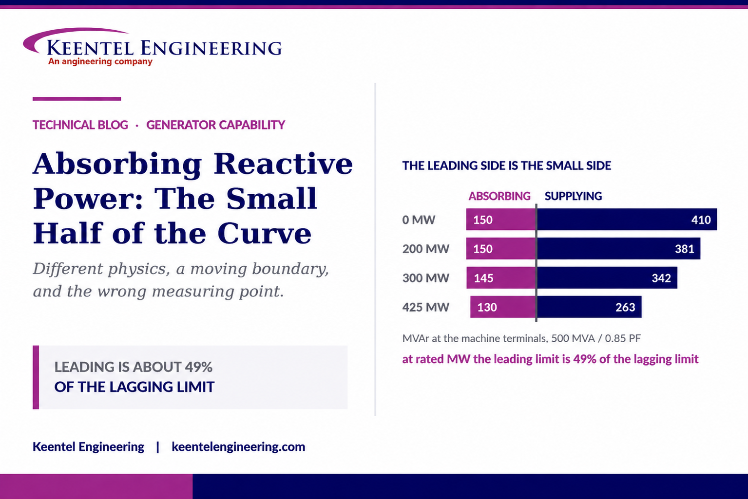
First, the leading region of a capability curve is roughly half the size of the lagging region, and it is limited by different physics. For a representative 500 MVA, 0.85 power factor, hydrogen-cooled turbogenerator, the lagging boundary at rated real power is about 263 MVAr, set by field current. The leading boundary at the same real power is about 130 MVAr around forty-nine percent of it and it is set by heating in the stator core end region, not by any current the operator can see on a meter.
Second, the capability curve is not a fixed boundary. It is drawn at one terminal voltage, one hydrogen pressure and one cold-gas temperature. Drop the terminal voltage from 1.00 to 0.90 per unit and the same machine loses about fourteen percent of its lagging capability at rated real power. Operate at reduced hydrogen pressure and it loses more. None of this is visible on the single laminated curve taped to the control room wall.
Third and this is the finding that most often surprises a plant owner the generator step-up transformer consumes a large fraction of the lagging capability and gives leading capability away for free. For the same machine with a twelve percent GSU, the transformer absorbs about 60 MVAr at the rated lagging point. That is roughly twenty-three percent of the declared lagging capability, gone between the machine terminals and the high side. On the leading side the sign reverses and the plant delivers about thirty-seven percent more absorption at the high side than the machine itself is producing. Reactive capability is not a property of the generator. It is a property of the generator, the step-up, the tap position, the auxiliary load and the measuring point taken together.
Fourth, the margin between legitimate absorption and the loss-of-field relay is narrowest at low real power precisely the condition in which a lightly loaded line demands the deepest absorption. For a correctly set two-zone characteristic on the representative machine, the separation between the end-region thermal limit and the zone 2 pickup is about 187 MVAr at rated real power and about 107 MVAr at zero real power. A setting derived on the wrong machine base can close most of that.
The sentence worth taking from this
A generator's reactive capability is not a number on a nameplate. It is a boundary that moves with terminal voltage, cooling and real power, measured at a point that is not the machine terminals, and enforced by limiters and relays that have to be set against it.
Every one of those four things is a place where declared capability and delivered capability separate — and each separation is quantifiable before it is discovered in service.
2. Why a Lightly Loaded Line Pushes Reactive Power Back
The starting point is a piece of physics that is easy to state and easy to underestimate. An overhead transmission line is not only a series impedance. It is also a distributed capacitance between each conductor and ground, and between conductors. That capacitance is charged and discharged twice per cycle whether or not any real power is flowing, and charging a capacitance means generating reactive power.
The reactive power a line generates by virtue of its shunt capacitance is, to a good approximation:
Qc = V² × Bc
where V is the line-to-line voltage and Bc is the total shunt susceptance of the line. The reactive power the line consumes in its series reactance is:
Ql = 3 × I² × Xl
The first term depends on voltage and does not care about loading. The second depends on current squared and therefore rises very rapidly with loading. A line is a reactive source at light load and a reactive sink at heavy load, and there is a crossover between the two.
Numbers make this concrete. Take a representative 345 kV double-bundled line with a series reactance of about 0.588 ohms per mile and a shunt susceptance of about 7.2 microsiemens per mile. A 120 mile length of it has a total shunt susceptance of 864 microsiemens and a series reactance of 70.6 ohms. At nominal voltage that line generates about 103 MVAr from its capacitance alone, before a single megawatt is transferred.
| Real power flow (MW) | Fraction of SIL | Q generated (MVAr) | Q consumed (MVAr) | Net to the system |
|---|---|---|---|---|
| 0 | 0.00 | 103 | 0 | +103 MVAr supplied |
| 100 | 0.24 | 103 | 6 | +97 MVAr supplied |
| 200 | 0.48 | 103 | 24 | +79 MVAr supplied |
| 300 | 0.72 | 103 | 53 | +50 MVAr supplied |
| 417 | 1.00 | 103 | 103 | zero — exact balance |
| 500 | 1.20 | 103 | 148 | −45 MVAr absorbed |
| 600 | 1.44 | 103 | 213 | −111 MVAr absorbed |
| 800 | 1.92 | 103 | 379 | −277 MVAr absorbed |
Somebody has to take the surplus at the light-load end of that table. If nothing absorbs it, it charges the system capacitance further, voltage rises, and because the generated reactive power goes as voltage squared, the surplus grows again. It is a positively reinforcing process, and left alone it does not settle at a comfortable value.
In practice the surplus is taken by shunt reactors where they are installed, by underexcited generators where they are not, and by whatever combination of the two the operating plan specifies. On a system without sufficient reactor capacity, the generator is the control of last resort, and it is asked to operate in the smallest and least understood part of its capability.
Underground cable makes the same problem an order of magnitude worse
A high-voltage cable has roughly twenty to fifty times the shunt capacitance per unit length of an equivalent overhead line, because the conductor and the screen are separated by millimetres of dielectric rather than metres of air.
A few miles of transmission cable can therefore generate as much reactive power as a hundred miles of overhead line. Urban and generator-lead cable sections are a common and frequently underestimated source of light-load reactive surplus.
3. Surge Impedance Loading: The Pivot of the Whole Problem
The crossover in the table above is not a coincidence and it is not specific to that line. It is the surge impedance loading, and it is the single most useful number for reasoning about which way a line leans.
The surge impedance, sometimes called the characteristic impedance, is the square root of the ratio of series reactance to shunt susceptance:
Zc = √( x / b )
and the surge impedance loading is the real power transfer at which the line, operated at nominal voltage, consumes in its series reactance exactly what it generates in its shunt capacitance:
SIL = V² / Zc
Below the surge impedance loading, a line is a net reactive source. Above it, a net reactive sink. At it, the line is reactively self-sufficient and its voltage profile is flat from end to end. That is an exact result for a lossless line and a very good approximation for a real one.
| Nominal voltage | Typical Zc (ohms) | Approximate SIL (MW) | Charging per 100 miles (MVAr) |
|---|---|---|---|
| 138 kV | 390 | 49 | 10 |
| 230 kV | 309 | 171 | 34 |
| 345 kV | 286 | 417 | 86 |
| 500 kV | 260 | 962 | 200 |
| 765 kV | 236 | 2,483 | 527 |
Two things in that table are worth pausing on. The surge impedance barely changes across the whole voltage range — it is set by conductor geometry, and bundling brings it down modestly. Surge impedance loading therefore scales essentially with the square of voltage, which is why a 765 kV line carries roughly fifty times the natural loading of a 138 kV line.
The charging column scales the same way, and that is the operational consequence. A 200 mile 500 kV line generates around 400 MVAr at nominal voltage. It is entirely normal for such a line to require dedicated shunt reactors sized in the hundreds of MVAr simply to be energised without the far-end voltage going out of range.
For anyone assessing a reactive problem quickly, surge impedance loading is the first number to compute. A plant operating persistently below the surge impedance loading of its outlet lines will be asked to absorb. A plant operating persistently above it will be asked to supply. That single ratio predicts which half of the capability curve the machine is going to live in, and therefore which half needs to be studied properly.
4. The Ferranti Effect, With Numbers
The named phenomenon behind all of this is the Ferranti effect: on a lightly loaded or open-ended transmission line, the receiving-end voltage is higher than the sending-end voltage. It is counter-intuitive on first encounter, because intuition says that a line drops voltage.
The mechanism is that the charging current of the line's shunt capacitance flows through the line's own series inductance. A capacitive current leading the voltage by ninety degrees, flowing through an inductive reactance, produces a voltage rise rather than a drop. With no load at the far end the entire charging current flows through the whole series reactance, and the rise is at its maximum.
For a lossless line, the open-circuit voltage ratio has a compact closed form:
Vr / Vs = 1 / cos( β ℓ )
where Vr and Vs are the receiving-end and sending-end voltages, β is the phase constant in radians per unit length, and ℓ is the line length. For the representative 345 kV line above, β works out to 0.1179 degrees per mile. That produces the following open-end rises.
| Line length | Electrical length βℓ | Voltage ratio | Rise |
|---|---|---|---|
| 50 miles | 5.89° | 1.0053 | +0.5% |
| 100 miles | 11.79° | 1.0215 | +2.2% |
| 150 miles | 17.68° | 1.0496 | +5.0% |
| 200 miles | 23.58° | 1.0911 | +9.1% |
| 250 miles | 29.47° | 1.1486 | +14.9% |
| 300 miles | 35.37° | 1.2263 | +22.6% |
The non-linearity is the point. At 100 miles the rise is a couple of percent — a nuisance. At 200 miles it is nine percent, which on a 345 kV system takes an already high bus straight out of the normal operating range. At 300 miles it is twenty-three percent, which is an equipment protection question rather than a voltage schedule question.
Two operational cases deserve specific attention. The first is line energisation, where a line is closed at one end before being closed at the other; the open end sees the full Ferranti rise, and the energising source sees a large capacitive inrush. The second is load rejection, where a line that was carrying substantial power suddenly is not; the series consumption vanishes in a cycle and the charging does not, leaving a large reactive surplus and a fast voltage rise that the excitation system has to catch.
Why this lands on the generator
Shunt reactors are fixed, or switched in discrete blocks. A generator's excitation system is continuous and fast. Where the required absorption changes hour by hour, only the machine can follow it.
That is why absorption duty concentrates on the units electrically closest to the lightly loaded lines, and why those units are the ones that need their leading capability studied rather than assumed.
5. Absorbing Is Not Simply the Reverse of Supplying
The convenient mental model — that supplying and absorbing reactive power are the same operation with the sign flipped — is where most of the trouble starts. They are not symmetric, in three separate respects.
The physical mechanism is different
To supply reactive power, the machine is overexcited. Field current is raised, the internal voltage behind synchronous reactance exceeds the terminal voltage, and reactive power flows out. The limiting factor is heat in the field winding, because the operator is adding field current.
To absorb reactive power, the machine is underexcited. Field current is reduced, the internal voltage falls below the terminal voltage, and reactive power flows in. The limiting factor is not heat in the field winding field current is being reduced, so the rotor is getting cooler. The limiting factor is heat somewhere else entirely: in the stator core end region, where flux that the field would normally suppress is now free to enter the end laminations and the structural steel.
The operator has less room
Because the two boundaries are set by different physics, they are not at symmetric distances from the axis. For almost every large synchronous machine the leading region is substantially smaller than the lagging region — commonly in the range of a third to a half.
The consequences of hitting the boundary are different
Overexcite too far and the overexcitation limiter acts, then the field overload protection; the machine gets hot slowly and the protection has time to work. Underexcite too far and the possible outcomes include end-region overheating that is not directly measured, and loss of synchronism, which is fast. The leading side is the side where the machine can lose step.
| Supplying (overexcited, lagging) | Absorbing (underexcited, leading) | |
|---|---|---|
| Field current | Increased | Reduced |
| Internal voltage vs terminal | Higher | Lower |
| Binding thermal limit | Rotor field winding | Stator core end region |
| Is it directly measured? | Yes — field current and rotor temperature | Rarely — end-region temperature is usually inferred |
| Stability consequence | None; the machine is well-held | Approaches the steady-state stability limit |
| Limiter | Overexcitation limiter (OEL) | Underexcitation limiter (UEL) |
| Backup protection | Field overload (ANSI 76 / 24 interaction) | Loss of field (ANSI 40) |
| Typical size at rated MW | 100% reference | Roughly 35% to 55% of the lagging value |
That last row is the reason a plant that has never had difficulty meeting a lagging voltage schedule can discover, the first time it is asked to absorb, that it does not have the room it assumed.
6. The Capability Curve: Three Limits, Three Different Physics
The reactive capability curve — the D-curve, in common usage — is a plot of real power on one axis against reactive power on the other, with a boundary enclosing the permissible continuous operating region. It looks like a single shape. It is three separate constraints, each from unrelated physics, and the boundary is the innermost of them at every point.
The three arcs
Moving around the boundary from the lagging side to the leading side, the three constraints are:
- The rotor (field current) limit, which bounds the lagging region. It is an arc of a circle whose centre is displaced from the origin along the reactive axis.
- The stator (armature current) limit, which bounds the high-real-power region. It is an arc of a circle centred on the origin, because armature current is proportional to total apparent power.
- The underexcited limit, which bounds the leading region. On large cylindrical-rotor machines this is set by end-region heating; on smaller and salient-pole machines it is often set by steady-state stability instead.
Where they meet
There is a design elegance worth pointing out, because it is a useful check on any curve handed to you. On a well-matched machine, the rotor and stator limits intersect exactly at the nameplate rating point. For a 500 MVA machine at 0.85 power factor, that point is 425 MW and 263.4 MVAr. The rotor arc and the stator arc both pass through it. That is not accidental: the machine is designed so that rated field current and rated armature current are reached simultaneously at the nameplate condition. Neither is wasted.
Away from that point they diverge, and which one binds changes. Below rated real power, the field limit is the tighter of the two. Above it, the stator limit takes over.
| Real power (MW) | Rotor limit allows (MVAr) | Stator limit allows (MVAr) | Binding constraint |
|---|---|---|---|
| 0 | 410 | 500 | Rotor (field current) |
| 100 | 403 | 490 | Rotor |
| 200 | 381 | 458 | Rotor |
| 300 | 342 | 400 | Rotor |
| 400 | 282 | 300 | Rotor |
| 425 (rated) | 263 | 263 | Both — the design point |
| 450 | 243 | 218 | Stator (armature current) |
The first row of that table contains a result that is routinely got wrong. At zero real power — a synchronous condenser operating mode, or a unit held on line at minimum load — the lagging capability is not the machine's full MVA rating. The stator would permit 500 MVAr, but the field will only sustain 410. The difference, eighteen percent, is often assumed away when reactive resources are counted in a planning study.
A quick sanity check on any capability curve
Confirm the rotor and stator arcs intersect at the nameplate MW and MVAr. If they do not, either the curve has been redrawn for a non-standard condition, or the machine has been rerated, or the plot is wrong.
Confirm the zero-real-power lagging intercept is below the MVA rating. If the curve shows a flat MVA-rated boundary all the way to zero real power, the field limit has been omitted.
7. The Stator Limit — Armature Current and Total MVA
This is the most intuitive of the three, and the only one that needs little explanation. Current in the armature winding produces resistive loss, the loss produces heat, and the insulation system has a temperature limit. The permissible continuous armature current follows from the winding's thermal class and the cooling system.
Because apparent power at the terminals is the product of terminal voltage and armature current, and because the voltage is normally held close to constant, an armature current limit is a total MVA limit:
P² + Q² ≤ Srated²
which plots as a circle of radius Srated centred on the origin. It bounds the top of the curve, and by symmetry it applies equally to the lagging and the leading side.
Two subtleties deserve a note.
The first is that the limit is on current, not on apparent power. If terminal voltage falls, the same armature current corresponds to less MVA. A machine operated at 0.95 per unit terminal voltage has an MVA-equivalent stator limit five percent below nameplate, exactly in proportion. This is one of several reasons the capability curve moves with voltage.
The second is that the armature limit is a continuous rating and is defined at a specified coolant inlet temperature. Short-time overload capability exists and is defined in the machine standards, but it is not part of the continuous capability envelope and should not be counted in steady-state reactive planning.
8. The Rotor Limit — Field Current and the Lagging Boundary
The lagging boundary is a field current limit, and the geometry that produces it is worth deriving because it explains the shape.
For a round-rotor machine, neglecting saliency and resistance, the real and reactive power at the terminals are:
P = ( Vt · E / Xd ) · sin δ Q = ( Vt · E / Xd ) · cos δ − Vt² / Xd
where Vt is the terminal voltage, E is the internal voltage behind synchronous reactance, Xd is the saturated direct-axis synchronous reactance, and δ is the rotor angle. Eliminating δ between the two gives:
P² + ( Q + Vt² / Xd )² = ( Vt · E / Xd )²
which is a circle. Its centre sits on the reactive axis at minus Vt squared over Xd, and its radius is proportional to the internal voltage — that is, proportional to field current. Fixing the field current at its maximum continuous value fixes the radius, and the resulting arc is the lagging boundary.
For the representative machine, with a saturated synchronous reactance of 1.8 per unit and rated terminal voltage, the centre lies at −0.556 per unit and the radius is 1.376 per unit, corresponding to a maximum internal voltage of about 2.48 per unit. Those three numbers reproduce the entire lagging boundary.
Why the arc leans the way it does
The centre of the field circle sits below the origin, at a distance that depends only on terminal voltage and synchronous reactance. The physical meaning of that offset is the reactive power the machine absorbs with the field completely removed the magnetising requirement of the machine itself. Everything the field does is measured from there, not from zero.
This also explains why a machine with a lower synchronous reactance has a lagging boundary further from the origin, and why the same machine at reduced terminal voltage loses lagging capability faster than the voltage reduction alone would suggest both the centre and the radius move.
What actually limits field current
Field winding temperature, measured or inferred from field resistance, is the direct constraint. Behind it sit the exciter's continuous rating and, on machines with brushes, the collector ring and brush gear. On a brushless machine the rotating rectifier assembly has its own rating. A plant that has replaced an exciter, or is operating one that has degraded, may have a field limit well below what the original capability curve shows — and this is a common and entirely unglamorous reason for a MOD-025 shortfall.
9. The Leading Region — End-Region Heating and the Small Side
This is the section that matters most, because it covers the part of the curve that is smallest, least measured and most often assumed.
The mechanism
In a large cylindrical-rotor generator, the stator core is a stack of thin laminations. At the two ends of the stack, the magnetic circuit is not closed in the way it is in the middle; flux escapes axially into the end laminations, the clamping fingers, the core-end flange and the surrounding structural steel. Those components are not laminated in the plane of that flux, so the eddy currents it induces have a low-resistance path and they dissipate real heat.
When the machine is overexcited, the rotor field produces a large direct-axis flux that partially opposes and suppresses this end leakage. When the machine is underexcited, that suppression is removed. The retaining ring at the end of the rotor becomes more heavily saturated, and the end-region flux rises. The heating is concentrated in a few localised spots in the core end and the clamping structure.
Three things make this limit difficult to manage in practice:
- It is usually not directly measured. Stator winding resistance temperature detectors are in the slots, in the middle of the core, and they see very little of it. Some machines have core-end thermocouples; many do not.
- It gets worse as terminal voltage rises, because the end-region flux depends on terminal voltage. That is the opposite of the lagging limit, which gets worse as voltage falls. The leading boundary and the lagging boundary move in opposite directions with voltage.
- It is strongly machine-specific. It depends on the end-region flux shielding design, the retaining ring material — magnetic versus non-magnetic — and the cooling arrangement at the core end. Two machines with identical nameplates from different manufacturers can have materially different leading capability.
How much smaller is the leading side?
For the representative machine, a leading boundary of around 130 MVAr at rated real power is consistent with a well-designed hydrogen-cooled unit. Against the 263 MVAr lagging boundary at the same real power, that is 49 percent. Expressed as a power factor, the machine is capable of about 0.85 lagging and about 0.956 leading at the same 425 MW.
| Real power (MW) | Leading limit (MVAr) | Apparent power (MVA) | Power factor leading |
|---|---|---|---|
| 0 | −150 | 150 | 0 (pure absorption) |
| 100 | −150 | 180 | 0.555 |
| 212 | −150 | 260 | 0.816 |
| 300 | −145 | 333 | 0.900 |
| 340 | −140 | 368 | 0.925 |
| 425 (rated) | −130 | 444 | 0.956 |
Note the shape. The leading boundary is relatively flat and then tapers as real power rises. It does not scale with apparent power the way the stator limit does, because end-region heating is driven by flux and by the combination of terminal voltage and underexcitation, not by total current.
Why a magnetic retaining ring matters
Older machines were commonly built with magnetic retaining rings, which carry end-region flux and heat readily. Many were later refitted with non-magnetic rings — typically an 18Mn-18Cr austenitic alloy — primarily to address stress corrosion cracking.
A frequent and welcome side effect of that refit is improved underexcited capability, because the non-magnetic ring does not concentrate end-region flux in the same way. If a machine has had a rotor rewind or a retaining ring replacement, its original leading capability curve may now be conservative — but only a test will establish by how much.
10. Steady-State Stability: The Limit That Moves With the System
End-region heating is a thermal limit and belongs to the machine. Steady-state stability is an electromechanical limit and belongs to the machine and the network together. The distinction matters because one of them moves when the system changes and the other does not.
A synchronous machine holds synchronism through the restoring torque produced when the rotor angle increases. That restoring torque reaches a maximum at ninety degrees of angle across the total reactance from the internal voltage to the system, and beyond it the machine pulls out of step. Reducing excitation reduces the internal voltage, which reduces the maximum transferable power, which brings that pull-out condition closer. Underexcited operation therefore erodes stability margin directly.
Plotted on the machine terminal P-Q plane, the steady-state stability limit is another circle. Including the external reactance from the terminals to the system — the step-up transformer plus the system equivalent the circle has:
centre = ( Vt² / 2 ) · ( 1/Xe − 1/Xd ) radius = ( Vt² / 2 ) · ( 1/Xe + 1/Xd )
There is a result hidden in that pair of expressions that is worth stating plainly. At zero real power, the stability limit is always minus Vt squared over Xd, regardless of the external reactance. The external system does not affect the zero-load stability limit at all. What it affects is how quickly the limit closes in as real power rises.
| System equivalent reactance | Total external Xe | Stability limit at 0 MW | Stability limit at 425 MW |
|---|---|---|---|
| 0.05 pu (very strong) | 0.17 pu | −278 MVAr | −221 MVAr |
| 0.10 pu (strong) | 0.22 pu | −278 MVAr | −205 MVAr |
| 0.20 pu (moderate) | 0.32 pu | −278 MVAr | −174 MVAr |
| 0.35 pu (weak) | 0.47 pu | −278 MVAr | −126 MVAr |
| 0.50 pu (very weak) | 0.62 pu | −278 MVAr | −72 MVAr |
Read the last two rows against the end-region limit of 130 MVAr at rated real power. On a strong system, the thermal limit binds first, with around 75 MVAr of margin to the stability limit. On a weak system — one line out of service, a remote plant, an outage season configuration the stability limit crosses inside the thermal limit and becomes the governing constraint.
This is the single most important reason that a leading capability study cannot be done on the machine alone. The capability curve is fixed. The stability boundary is not, and it can move inside the curve when the network changes. A unit whose underexcitation limiter was set against a normal-system stability limit can be left without margin in a contingency configuration.
In practice the operating limit is set with margin against the theoretical boundary commonly a real power margin of around ten percent, or an equivalent reactive margin and the limiter is then set against that. The margin exists because the theoretical limit assumes a constant internal voltage and no dynamics, and the real machine has an excitation system that is trying to respond.
11. The Curve Is Drawn at One Operating Condition
A capability curve is a photograph, not a law. Every one of them is drawn at a stated terminal voltage, a stated coolant condition and a stated ambient. Change any of those and the curve changes, sometimes substantially. The stated conditions are printed on the curve, and they are the part most often not read.
Terminal voltage
Both the stator limit and the rotor limit scale with terminal voltage, and they do not scale by the same amount.
| Terminal voltage (pu) | Stator MVA limit | Change | Lagging limit at 425 MW | Change |
|---|---|---|---|---|
| 1.05 | 525 MVA | +5.0% | 278 MVAr | +5.6% |
| 1.00 (reference) | 500 MVA | — | 263 MVAr | — |
| 0.95 | 475 MVA | −5.0% | 246 MVAr | −6.6% |
| 0.90 | 450 MVA | −10.0% | 225 MVAr | −14.4% |
The lagging capability falls faster than the voltage, because both the centre and the radius of the field circle depend on terminal voltage. At 0.90 per unit the machine has lost more than fourteen percent of its lagging capability. That is the worst possible timing: low terminal voltage is exactly the condition in which the system is asking for more lagging reactive power, and it is exactly the condition in which the machine has less to give. Reactive support is a positively unstable resource in this sense, and it is the core of the voltage collapse mechanism.
On the leading side the direction reverses. Higher terminal voltage drives more end-region flux and reduces underexcited capability. A machine held at 1.05 per unit may have roughly ten percent less leading capability than the same machine at nominal. Absorbing duty and high terminal voltage work against each other.
Hydrogen pressure
On a hydrogen-cooled machine, the cooling capacity depends on gas density and therefore on pressure. Machine ratings are quoted at a stated pressure, and operation at a lower pressure carries a defined derating. Typical published multipliers follow a pattern of this kind, although the actual values are always machine-specific:
| Hydrogen pressure | Approximate MVA multiplier | Derated MVA (from 500) | Lagging at rated MW |
|---|---|---|---|
| 75 psig | 1.00 | 500 MVA | 263 MVAr |
| 60 psig | 0.95 | 475 MVA | 250 MVAr |
| 45 psig | 0.89 | 445 MVA | 234 MVAr |
| 30 psig | 0.82 | 410 MVA | 216 MVAr |
| 15 psig | 0.74 | 370 MVA | 195 MVAr |
| Air (purged) | 0.60 – 0.70 | 300 – 350 MVA | 158 – 184 MVAr |
A plant running at reduced hydrogen pressure because of a seal leak it has not yet repaired is operating on a smaller capability curve than the one on the wall, and it has usually not told its reliability coordinator.
Cold gas and ambient temperature
Capability is also stated at a cold-gas temperature, typically in the region of 40 to 46 degrees Celsius for hydrogen-cooled machines. Higher cooler water temperature, fouled hydrogen coolers, or a hot summer on an air-cooled machine all reduce the available capability. The effect is usually modest compared with hydrogen pressure but it is real, and it correlates with summer peak conditions.
The three questions to ask of any capability curve
At what terminal voltage was it drawn, and is that the voltage the unit actually runs at?
At what hydrogen pressure and cold-gas temperature, and is that the condition the unit actually operates in?
What is the date, and has the machine been rewound, refitted with a different retaining ring, or had its exciter replaced since?
12. Q at the Machine Is Not Q at the Point of Interconnection
Every number discussed so far has been at the generator terminals. Every obligation a plant has is at the point of interconnection. Between the two sits the generator step-up transformer, and it consumes reactive power in proportion to the square of the current through it.
Qgsu = I² × Xt or in per unit, Qgsu = ( S / Srated )² × Xt
For the representative 500 MVA machine with a twelve percent GSU on the same base, the consequences are large and they are asymmetric.
| Operating point at the machine | Apparent power | GSU consumes | Q at the high side | Change |
|---|---|---|---|---|
| 425 MW, +263 MVAr (max lagging) | 500 MVA | 60.0 MVAr | +203 MVAr | −23% |
| 300 MW, +342 MVAr (max lagging) | 455 MVA | 49.6 MVAr | +292 MVAr | −15% |
| 0 MW, +410 MVAr (max lagging) | 410 MVA | 40.4 MVAr | +370 MVAr | −10% |
| 425 MW, −130 MVAr (max leading) | 444 MVA | 47.4 MVAr | −177 MVAr | +37% |
| 300 MW, −145 MVAr (max leading) | 333 MVA | 26.6 MVAr | −172 MVAr | +18% |
| 0 MW, −150 MVAr (max leading) | 150 MVA | 5.4 MVAr | −155 MVAr | +4% |
Three conclusions follow from that table and they are worth stating separately.
The step-up transformer eats lagging capability. At the rated lagging point, 60 of the 263 MVAr the machine produces never leave the plant. Twenty-three percent of the declared capability is consumed internally. If the number a planning model uses at the point of interconnection came from the machine's terminal capability curve, that model believes the plant can hold a voltage it physically cannot hold.
The step-up transformer gives leading capability away. At the maximum leading point the plant delivers 177 MVAr of absorption at the high side while the machine is only absorbing 130. Thirty-seven percent more absorption reaches the system than the machine produces. A plant that is short on lagging support at the point of interconnection is frequently comfortable on leading, and the reverse is rarely true.
The asymmetry gets worse as the plant gets busier. Because the loss goes as current squared, it is at its worst exactly at full output, which is when the obligation is usually tested.
What the obligation actually requires
The standard interconnection design criterion in North America is a power factor range of 0.95 leading to 0.95 lagging, measured at the point of interconnection, at continuous rated real power. That translates into specific MVAr quantities:
| Real power at the POI | MVAr required for 0.95 PF | MVAr the machine must produce | Rotor limit allows |
|---|---|---|---|
| 425 MW | ±140 MVAr | 192 MVAr lagging | 263 MVAr — meets |
| 340 MW | ±112 MVAr | 145 MVAr lagging | 321 MVAr — meets |
| 255 MW | ±84 MVAr | 102 MVAr lagging | 361 MVAr — meets |
| 170 MW | ±56 MVAr | 64 MVAr lagging | 389 MVAr — meets |
The representative machine meets the obligation comfortably at nominal conditions. Now degrade the conditions: terminal voltage at 0.95 per unit and hydrogen pressure reduced enough to cost eight percent of rating. The requirement at the machine is unchanged at 192 MVAr; the available lagging capability falls to about 226 MVAr. The margin has gone from 71 MVAr to 34 MVAr still passing, but now inside the range of ordinary measurement uncertainty and ordinary equipment degradation.
Tap position and auxiliary load
Two further items complete the picture. The GSU tap position sets the relationship between the machine terminal voltage and the high-side voltage; a tap chosen for a historical voltage profile may force the machine to operate at a terminal voltage that costs it capability. And station service load commonly two to five percent of plant output in real power with an associated reactive component is subtracted somewhere, and exactly where depends on whether the auxiliary transformer is a unit auxiliary transformer tapped off the isolated phase bus or a station service transformer fed from the high side.
For the representative machine with an 18 MW, 9 MVAr auxiliary load, the maximum lagging point reads 263 MVAr at the machine terminals, 203 MVAr at the high side of the GSU, and 194 MVAr net of station service. Three defensible numbers for the same operating point. Which one belongs on a registration form depends entirely on what the form is asking for, and getting that wrong is one of the most common data-quality findings in reactive capability verification.
13. Limiters and Protection: UEL, OEL and Device 40
A capability curve is a statement about what the machine can do. Limiters and protection are what keep it there. The relationship between the three has to be deliberately engineered, and it is frequently not.
The ordering principle
On the leading side of the P-Q plane, moving outward from normal operation toward deeper absorption, the correct order is:
- Normal operating range — set by the voltage schedule.
- The underexcitation limiter (UEL) characteristic — a control function in the excitation system that acts to raise field current before a limit is reached. It should sit inside both the thermal capability boundary and the stability boundary, with margin.
- The machine capability boundary — end-region heating, or stability, whichever is inner at that real power.
- The steady-state stability limit for the prevailing network configuration.
- The loss-of-field relay (ANSI device 40) characteristic — protection, which must not operate for any condition the limiter is supposed to hold.
The UEL is a control action; it pushes the operating point back. The device 40 element is protection; it trips. If they are in the wrong order, a machine can be tripped for an operating condition it was instructed to be in.
The loss-of-field element and where it sits
The conventional loss-of-field scheme is two offset mho characteristics in the impedance plane, both offset downward by half the transient reactance:
- Zone 1: diameter 1.0 per unit on the machine base, short time delay of the order of 0.1 seconds. This catches a complete and rapid loss of excitation.
- Zone 2: diameter equal to the synchronous reactance Xd, longer time delay of the order of 0.5 to 0.6 seconds. This catches a slower partial loss.
For the representative machine at 22 kV and 500 MVA, the base impedance is 0.968 ohms. The synchronous reactance of 1.8 per unit is 1.742 ohms and the transient reactance of 0.30 per unit is 0.290 ohms. Zone 2 is therefore a 1.742 ohm diameter circle offset 0.145 ohms below the R axis.
Mapping that circle back into the P-Q plane gives the reactive power at which a legitimate operating point would enter the protection:
| Real power (MW) | End-region limit | Zone 2 pickup | Margin between them |
|---|---|---|---|
| 0 | −150 MVAr | −257 MVAr | 107 MVAr |
| 50 | −150 MVAr | −257 MVAr | 107 MVAr |
| 100 | −150 MVAr | −260 MVAr | 110 MVAr |
| 150 | −150 MVAr | −264 MVAr | 114 MVAr |
| 212 | −150 MVAr | −271 MVAr | 121 MVAr |
| 300 | −145 MVAr | −286 MVAr | 141 MVAr |
| 425 | −130 MVAr | −317 MVAr | 187 MVAr |
A correctly set element has comfortable margin everywhere. But note where the margin is smallest: at low real power. It falls from 187 MVAr at rated output to 107 MVAr at zero output — a forty-three percent reduction. Low real power is exactly the condition in which the lightly loaded line demands the deepest absorption. The protection is closest to legitimate operation at the moment the machine is most likely to be pushed toward it.
What a mis-set element does to that margin
Because the reach is specified in per unit of machine base impedance, an error in the base used to derive the setting translates directly into a reach error.
| Setting case | Zone 2 pickup at 0 MW | Zone 2 pickup at 150 MW | Margin at 150 MW |
|---|---|---|---|
| Correct: diameter Xd, offset Xd'/2 | −257 MVAr | −264 MVAr | 114 MVAr |
| Offset omitted | −278 MVAr | −278 MVAr | 128 MVAr |
| Diameter derived on a 700 MVA base | −348 MVAr | −356 MVAr | 206 MVAr |
| Diameter derived on a 350 MVA base | −184 MVAr | −191 MVAr | 41 MVAr |
The last row is the dangerous one. A reach derived on a machine base smaller than the actual machine which happens when a plant is uprated, when a relay setting is copied from a sister unit, or when a replacement relay is programmed from a legacy setting sheet without rebasing collapses the margin from 114 MVAr to 41 MVAr. At that point an ordinary dispatcher instruction to absorb, combined with a UEL that is slightly slow or out of service, can operate a trip element on a perfectly healthy machine.
The overexcitation side
The lagging side has the same structure and is generally better behaved. The overexcitation limiter acts on a time-inverse characteristic to bring field current back below the continuous rating after a permitted short-time excursion, and it must coordinate with the field overload protection above it and with the machine's short-time field thermal capability. The volts-per-hertz limiter and the 24 element sit alongside, protecting against overfluxing at low speed or high voltage. These functions are defined in the excitation system model standards and should be represented explicitly in any dynamic study a model that omits the limiters will show reactive support the plant will not actually deliver in a sustained event.
14. Verifying What You Declared: MOD-025-2 in Practice
In North America, generator reactive capability is not a matter of assertion. The reliability standard governing it requires generator owners to verify the real and reactive power capability of applicable units and to report the verified data to their transmission planner, on a recurring cycle. The equivalent obligation applies to synchronous condensers.
The testing is straightforward in principle and awkward in practice, because it requires the unit to be driven to its lagging and leading boundaries while connected to a live system that has its own voltage limits.
What a verification test actually involves
- Establishing the unit at a defined real power output, usually at or near maximum, and holding it there.
- Increasing excitation until a limit is reached — field current at its continuous rating, a stator or rotor temperature limit, the overexcitation limiter, or a system voltage constraint that prevents going further.
- Recording the sustained output at that point, with the associated terminal voltage, field current, hydrogen pressure, cold-gas temperature, ambient and station service load.
- Repeating in the underexcited direction until the leading limit is reached, with the same set of conditions recorded.
- Reporting the verified values, and documenting any limitation that prevented reaching the machine boundary.
Where these tests go wrong
The single most common outcome of a first verification test is not that the machine failed. It is that the test could not reach the machine's boundary because the system got in the way — the bus voltage hit its upper limit before the field reached its rating on the lagging test, or its lower limit on the leading test. That is a legitimate result and it must be documented as such, but it means the verified capability is a system-limited value rather than a machine value, and it should not be recorded as though the machine were the constraint.
The second most common finding is a mismatch in the measuring point, as described in the previous section. The machine terminal value, the high-side value and the net-of-auxiliaries value differ by tens of MVAr on a machine of this size, and the correct one depends on the definition in the reporting form.
The third is a condition mismatch. A test conducted at 0.98 per unit terminal voltage and 60 psig hydrogen on a cool day does not verify the capability available at 1.02 per unit and 45 psig on an August afternoon. Recording the conditions is not paperwork; it is what makes the number usable.
Test the leading direction properly, not as an afterthought
Leading tests are frequently curtailed because the operator is uncomfortable, because the low-voltage limit is reached, or because nobody is confident the underexcitation limiter and the loss-of-field element are correctly coordinated.
That discomfort is itself the finding. If a plant cannot confidently drive its own machine into the leading region, the coordination review should happen before the test, not instead of it.
15. When the Machine Is the Wrong Tool
There is an implicit assumption running through much of this subject that the generator is the natural place to put reactive duty. Often it is not, and the economics are not subtle.
Consider the 120 mile 345 kV line from section 2. It generates about 103 MVAr at nominal voltage, and about 113 MVAr at 1.05 per unit, because charging goes as voltage squared. If that absorption is assigned to a single generator with a leading capability of 130 MVAr, the line consumes seventy-nine percent of the machine's entire underexcited capability. There is nothing left for anything else no margin for a contingency, no room for a second line, no ability to respond to a disturbance.
Two 51 MVAr shunt reactors, one at each end, cancel the same charging with no operational cost and no thermal consequence for any rotating machine. They are not free, but they are a capital item rather than a permanent constraint on the flexibility of the generating unit.
| Device | What it does well | Principal limitation |
|---|---|---|
| Shunt reactor (line or bus connected) | Absorbs a fixed, large, cheap block of reactive power; ideal for cancelling known line charging | Fixed value; must be switched in discrete steps; switching duty on the breaker |
| Switched shunt capacitor | Supplies reactive power cheaply at defined steps | Output falls as voltage squared — weakest exactly when most needed |
| Generator excitation | Continuous, fast, already installed | Consumes capability that has other uses; limited and asymmetric leading range |
| Synchronous condenser | Continuous reactive in both directions plus inertia and short-circuit strength | Rotating plant with its own maintenance and auxiliary load |
| STATCOM | Fast, continuous, output current maintained at depressed voltage | Higher capital cost per MVAr; power electronics maintenance and harmonic considerations |
| SVC | Fast and continuous over a defined range | Output falls as voltage squared in the capacitive range; filter requirements |
The design question is not which device is best. It is which part of the reactive requirement is fixed and predictable, and which part is variable and fast. Fixed and predictable requirements belong on fixed equipment. Variable and fast requirements belong on the machine or on a dynamic device. Putting a fixed requirement on a machine is spending a scarce and flexible resource on a job that a cheap and inflexible one would do.
There is one further consideration that has grown in importance. As synchronous generation is displaced during high-renewable hours, the units remaining on line are asked to absorb more, for longer, at lower real power output. That is the deepest and most constrained part of the capability curve, and it is the part with the least margin to the protection. It is also where the reactive capability of inverter-based resources becomes directly relevant, because they are now subject to the same point-of-interconnection power factor obligation and can, when specified and commissioned properly, carry a meaningful share of that duty.
16. North American Practice, Units and Obligations
Much of the widely circulated material on this subject uses IEC conventions and metric units. The physics is identical, but the standards framework, the terminology and the compliance obligations in North America differ in ways that matter to anyone specifying, testing or registering a machine here.
Units and conventions
| Item | Common international usage | North American practice |
|---|---|---|
| Reactive power symbol and unit | Q in Mvar or kvar | Q in MVAr or kVAr; MVAR also seen |
| Sign convention | Varies; IEC load convention common | Generator convention: positive Q means supplying (overexcited, lagging) |
| Power factor description | Overexcited / underexcited | Lagging / leading, used interchangeably with over- and underexcited |
| Generator standards | IEC 60034 series | IEEE C50.13 (cylindrical rotor), IEEE C50.12 (salient pole) |
| Hydrogen pressure | bar or kPa gauge | psig |
| Cold gas temperature | Degrees Celsius | Degrees Celsius, occasionally Fahrenheit on older curves |
| Protection identification | IEC function codes | ANSI/IEEE C37.2 device numbers — 40 for loss of field, 24 for overfluxing |
| Line length | Kilometres | Miles; conductor spacing and clearances in feet and inches |
The obligations that apply
Four distinct requirements govern reactive capability for a generating facility interconnecting to the North American bulk electric system, and they are often conflated.
The interconnection design criterion. The standard large generator interconnection agreement requires the facility to maintain a composite power delivery at continuous rated power output at the point of interconnection within a power factor range of 0.95 leading to 0.95 lagging, unless the transmission provider has established a different requirement through study. The measuring point is the point of interconnection, which is why section 12 is not an academic exercise. Since 2016 this obligation has applied to non-synchronous generation on the same basis as synchronous, following the removal of the earlier exemption.
Capability verification. Generator owners must verify real and reactive power capability on a recurring cycle and report the verified data. This is the standard that turns the capability curve from a manufacturer's document into a reported, auditable number.
Model verification. Separate standards require verification of the excitation control system model and of the turbine-governor and load control model, so that the dynamic behaviour used in planning studies matches the plant. A capability curve says what the plant can do in steady state; the model says how it gets there, and both have to be right.
Voltage schedule compliance. The operating standard requires the generator to maintain the voltage schedule or reactive output directed by the transmission operator, and to notify the transmission operator promptly when the automatic voltage regulator is out of service or when reactive capability is reduced. That last obligation is the one that a plant running on reduced hydrogen pressure, or with a degraded exciter, most often overlooks.
The practical translation
A capability curve supplied with a machine built to IEC conventions is entirely valid, but it is not by itself a compliant submission here.
It has to be restated at the point of interconnection, at the conditions the unit actually operates in, in the sign convention the form uses, and supported by a test performed and documented to the applicable verification standard.
17. Three Case Studies from Composite Project Experience
The three studies that follow are composite illustrations. They are assembled from patterns that recur across many projects and are deliberately generalised. They do not describe any specific client, site, project, manufacturer, generating unit or utility, and no operating data from any particular facility is presented. They are included because each one shows a different way in which declared capability and delivered capability separate.
Case Study One — The Capability That Never Left the Plant
Situation
A thermal generating station with a single large synchronous unit was identified in a regional planning study as a key reactive resource for a load pocket. The planning model showed the plant holding the high-side bus within limits following the loss of a nearby line. The plant had recently completed a reactive capability verification and had reported a lagging capability consistent with its nameplate power factor.
What was found
The reported capability had been taken from the machine terminal capability curve and entered into the model as the plant's capability at the point of interconnection. No adjustment had been made for the generator step-up transformer.
Recomputing the plant's reactive output at the high side, at the operating point the contingency study relied on, showed that the step-up transformer consumed a little under a quarter of the reported lagging capability. Station service consumed a further increment. The plant's actual reactive delivery at the point of interconnection was materially below the figure the study had used.
A secondary finding compounded it. The step-up transformer tap had been set years earlier for a system voltage profile that had since changed. At the tap in service, achieving the required high-side voltage forced the machine to a terminal voltage below the one at which its capability curve had been drawn, which cost a further several percent of lagging capability.
Resolution
The reactive capability was restated at three defined points machine terminals, transformer high side, and net of station service with the conditions recorded for each, and the planning model was updated with the correct one. A tap study established a position that allowed the machine to operate closer to the terminal voltage its curve assumed. The combination recovered part of the shortfall; the remainder was addressed by the planner reassessing the reactive requirement of the load pocket with the corrected data.
What the case illustrates
The gap here was not caused by a bad machine, a bad test or a bad model. It was caused by a boundary-definition error: two parties using the same number to mean two different things. It is the most common reactive data problem in the industry and the cheapest one to fix, because fixing it requires arithmetic and a clear definition rather than any capital work.
Case Study Two — A Healthy Machine Tripped on Loss of Field
Situation
A generating unit was instructed by its system operator to absorb reactive power overnight to control a high-voltage condition on a lightly loaded transmission corridor. The unit was operating at reduced real power output, well below its rating, with a substantial leading reactive output. The loss-of-field protection operated and the unit tripped. There was no fault, no loss of excitation, and no abnormality found in the excitation system on subsequent inspection.
What was found
The review examined the coordination between the machine capability curve, the underexcitation limiter and the loss-of-field element, and found two independent problems that had combined.
The first was a settings error. The unit had been uprated some years earlier, and the loss-of-field element's zone 2 reach had been derived from the synchronous reactance expressed on the pre-uprate machine base. Applied to the larger machine, the reach was substantially longer in physical terms than intended. Mapping the characteristic into the real and reactive power plane showed that the margin between the machine's legitimate underexcited thermal limit and the relay pickup had collapsed to a fraction of its intended value.
The second was that the margin is at its smallest at low real power in any case. At full output the coordination would still have held even with the reach error. At the reduced real power the unit was operating at, it did not.
The underexcitation limiter was correctly set against the capability curve and had in fact acted but the operating point had already been inside the mis-set relay characteristic, and the relay's time delay expired first.
Resolution
The zone 2 reach was recalculated on the correct machine base and the characteristic re-plotted in the real and reactive power plane against the capability curve, the underexcitation limiter characteristic and the steady-state stability boundary for both normal and credible contingency network configurations. The limiter characteristic was adjusted to restore a defined margin to the relay at the low real power conditions the unit was being dispatched into, and a coordination drawing covering the whole leading region was issued as a controlled document so that future settings changes would be checked against it.
What the case illustrates
Loss-of-field settings are typically derived once, from the machine data available at the time, and then carried forward through relay replacements and plant modifications. A machine uprate changes the base impedance and therefore changes every per-unit setting derived from it. The failure mode does not appear at full load, which is where most testing is done. It appears at low load and deep absorption, which is the condition the machine is increasingly being asked to operate in.
Case Study Three — The Leading Test That Stopped Early
Situation
A generating unit undergoing periodic reactive capability verification completed its lagging test without difficulty and reached a value consistent with its capability curve. The leading test was terminated by plant staff before the declared leading capability was reached, after temperature indications in the stator core end region rose faster than expected.
What was found
The unit was an older cylindrical-rotor machine that had been in service for several decades. Its capability curve was the original document supplied with the machine.
Three contributing factors were identified. The unit was being held at a terminal voltage toward the upper end of its normal range, which increases end-region flux and reduces underexcited capability the opposite of the lagging case, where high terminal voltage helps. The hydrogen coolers had degraded, raising the cold-gas temperature above the value at which the capability curve was drawn. And instrumentation in the core end region was sparse, so the temperature rise was detected late and its distribution was uncertain.
None of these individually would have prevented the test from completing. Together they reduced the available leading capability below the declared value.
Resolution
The verified leading capability was reported at the value actually demonstrated, with the terminal voltage, hydrogen pressure and cold-gas temperature recorded, and the limiting condition documented explicitly as a machine thermal limitation rather than a system constraint. The cooler condition was addressed under the plant's maintenance programme, and additional core-end instrumentation was specified for the next major outage so that a future test could be taken to the boundary with confidence.
Separately, the reduction in declared leading capability was communicated to the transmission operator. Because the unit had been a designated absorbing resource for a nearby lightly loaded corridor, the reactive plan for that corridor was reassessed, and the shortfall was ultimately covered by a fixed shunt reactor rather than by continuing to place the duty on the machine.
What the case illustrates
An original capability curve is a statement about a new machine under stated conditions. Neither the machine nor the conditions stay the same. The leading region is where that gap opens first, because it is the region with the least instrumentation, the most condition sensitivity and the smallest margin. Testing it properly is uncomfortable, which is precisely why it is the region where declared and actual capability most often diverge.
18. A Practical Checklist for Reactive Capability
The following is the sequence used on a reactive capability assessment. It is ordered so that the cheap findings come first.
Establish the boundary
- Define the measuring point explicitly: machine terminals, generator step-up high side, or point of interconnection net of station service. Write it on every number.
- Obtain the step-up transformer impedance on a stated base, and the tap in service.
- Obtain the station service real and reactive load and confirm where it is connected.
Qualify the capability curve
- Record the terminal voltage, hydrogen pressure and cold-gas temperature at which the curve was drawn.
- Confirm the rotor and stator arcs intersect at the nameplate rating point.
- Confirm the zero-real-power lagging intercept is the field limit, not the MVA rating.
- Establish the machine's modification history — rewinds, retaining ring replacement, exciter replacement, uprates — and whether the curve predates any of it.
Compute the operating reality
- Restate the lagging and leading boundaries at the terminal voltage the unit actually runs at.
- Apply the cooling derating for the hydrogen pressure and cold-gas temperature actually maintained.
- Translate both boundaries through the step-up transformer to the required measuring point.
- Compare against the interconnection obligation at the real power output the obligation is defined at.
Check the leading region specifically
- Compute the steady-state stability boundary for the normal network configuration and for credible contingency configurations, and establish whether it moves inside the thermal boundary.
- Plot the underexcitation limiter characteristic, the capability boundary, the stability boundary and the loss-of-field characteristic on one real and reactive power diagram.
- Verify the coordination margin at low real power, not only at rated output.
- Confirm every per-unit protection setting is on the current machine base.
Close the loop
- Reconcile the computed values against the most recent verification test, and explain any difference.
- Confirm the values reported to the transmission planner match the values in the planning model.
- Confirm the excitation system model, including limiters, reproduces the computed boundaries in simulation.
- Establish a trigger for re-verification: any uprate, rewind, exciter change, cooling change or protection replacement.
19. Keentel Engineering Reactive Power and Generator Services
Keentel Engineering LLC is a United States power system engineering firm working across generation, transmission, substation and large-load interconnection. Reactive capability work sits at the intersection of machine engineering, protection and system studies, and it is one of the areas where a single discipline working alone reliably misses things which is why Keentel Engineering approaches it as one connected assessment rather than three separate scopes.
Reactive capability assessment and restatement
Keentel Engineering takes a machine capability curve, the step-up transformer data, the tap position, the station service load and the actual operating conditions, and produces the reactive capability at whichever measuring point matters machine terminals, transformer high side, or point of interconnection net of auxiliaries — with the conditions documented for each. Where the values reported to a planner differ from the values a model is using, Keentel Engineering identifies the gap and quantifies it.
MOD-025 verification support
Keentel Engineering prepares reactive capability verification test procedures, supports execution, and prepares the documentation. That includes establishing in advance whether the test is likely to be machine-limited or system-limited, so that the result is interpreted correctly, and reviewing the protection coordination before the leading test rather than discovering a problem during it.
Underexcitation limiter and loss-of-field coordination
Keentel Engineering produces the single diagram that this work ultimately depends on: the capability boundary, the steady-state stability boundary for normal and contingency network configurations, the underexcitation limiter characteristic and the loss-of-field relay characteristic, all plotted together in the real and reactive power plane, with margins stated at every real power level rather than only at rated output.
Excitation and generator model verification
Keentel Engineering develops and validates excitation system and generator models, including limiter representation, so that dynamic studies reproduce what the plant will actually deliver. Models that omit limiters overstate sustained reactive support, and that overstatement propagates into every study that uses them.
System reactive planning and device selection
Keentel Engineering performs the power flow and voltage stability work that determines how much reactive capability a system actually needs, where it needs it, and how much of it should be fixed rather than dynamic. That includes shunt reactor and capacitor sizing, line energisation and load rejection studies, and technical evaluation of dynamic alternatives where the duty justifies them.
Interconnection and compliance engineering
Keentel Engineering supports generator interconnection across the North American markets, including reactive power obligation compliance at the point of interconnection, registration data, planning model data submissions, and the studies that support them for synchronous plant, inverter-based resources and hybrid facilities alike.
20. Frequently Asked Technical Questions
1. What does it actually mean for a generator to absorb reactive power?
It means the machine is underexcited: field current has been reduced far enough that the internal voltage behind synchronous reactance is lower than the terminal voltage. Reactive power then flows into the machine rather than out of it, and the armature current leads the terminal voltage. Nothing is being consumed in the sense that real power is consumed — reactive power is exchanged, not dissipated — but the condition does produce real heating, in a different part of the machine than overexcited operation does.
2. Why does a lightly loaded line need reactive power absorbed at all?
A line has distributed shunt capacitance that generates reactive power in proportion to voltage squared, independent of how much power it is carrying, and series reactance that consumes reactive power in proportion to current squared. At light load the first dominates and the line is a net reactive source. That surplus has to go somewhere. If nothing absorbs it, voltage rises, which increases the surplus further, because generation goes as voltage squared.
3. What is surge impedance loading and why is it the useful number?
Surge impedance loading is the real power transfer at which a line's series reactive consumption exactly equals its shunt reactive generation. Below it a line supplies reactive power; above it the line absorbs. It is computed as nominal voltage squared divided by the surge impedance, where the surge impedance is the square root of series reactance over shunt susceptance. It is useful because it tells you in one number which half of the capability curve the connected machines are going to live in.
4. What is the Ferranti effect?
It is the rise in receiving-end voltage above sending-end voltage on a lightly loaded or open-ended transmission line. The line's capacitive charging current, leading the voltage by ninety degrees, flows through the line's series inductance and produces a voltage rise rather than a drop. For a lossless line the open-end ratio is one divided by the cosine of the electrical length. It is small on short lines and grows non-linearly — roughly two percent on a hundred-mile 345 kV line, and around nine percent at two hundred miles.
5. Why is the leading half of the capability curve smaller than the lagging half?
Because the two halves are limited by different physics. The lagging boundary is a field current limit, set by rotor winding heating. The leading boundary on a large cylindrical-rotor machine is set by heating in the stator core end region, where flux that the field would normally suppress enters the end laminations and structural steel and produces localised eddy-current heating. That mechanism binds much earlier. A leading capability of roughly a third to a half of the lagging value is typical.
6. What exactly is end-region heating?
At the two ends of the stator core stack, flux escapes axially into the end laminations, the clamping fingers and the surrounding structural steel. Those parts are not laminated in the plane of that flux, so eddy currents induced in them dissipate real heat in localised spots. Underexcited operation removes the direct-axis flux that would otherwise suppress this leakage, and the retaining ring saturates further, so the effect grows. It is difficult to manage because stator slot temperature detectors sit in the middle of the core and see very little of it.
7. Does terminal voltage change the capability curve?
Yes, and in opposite directions on the two halves. The stator MVA limit scales directly with terminal voltage. The lagging limit falls faster than the voltage, because both the centre and the radius of the field circle depend on it — a representative machine loses around fourteen percent of its lagging capability at 0.90 per unit terminal voltage. The leading limit moves the other way: higher terminal voltage increases end-region flux and reduces underexcited capability.
8. Does hydrogen pressure change the capability curve?
Substantially. Cooling capacity depends on gas density, so the machine rating is quoted at a stated pressure. Operating at reduced pressure carries a defined derating that the manufacturer publishes as a set of curves. Losing a third to a half of the rated pressure can cost ten to twenty percent of MVA rating. A unit running at reduced pressure because of an unrepaired seal leak is operating on a smaller curve than the one on the control room wall, and that reduction is normally reportable to the transmission operator.
9. Where should the rotor and stator limits intersect on a correctly drawn curve?
Exactly at the nameplate rating point — rated MW and rated MVAr at the nameplate power factor. Machines are designed so that rated field current and rated armature current are reached simultaneously there, so neither is wasted. If a curve does not show that intersection, it has either been redrawn for a non-standard condition, the machine has been rerated, or the plot is in error. It is a quick and reliable sanity check.
10. At zero real power, can a generator supply its full MVA rating as reactive power?
Almost never. The stator limit would permit it, but the field limit is tighter at low real power and it governs. For a representative 500 MVA machine at 0.85 power factor with a synchronous reactance of 1.8 per unit, the lagging capability at zero real power is around 410 MVAr rather than 500 — about eighteen percent less. Planning studies that count a unit's full MVA rating as available reactive support at minimum load are overstating the resource.
11. How much reactive capability does the step-up transformer consume?
It consumes reactive power in proportion to the square of the current through it, which for a twelve percent transformer at full apparent power is twelve percent of the machine base. On a 500 MVA machine that is 60 MVAr — roughly twenty-three percent of the lagging capability at the rated point. The loss is worst at full output, which is when the interconnection obligation is usually tested.
12. Does the step-up transformer also reduce leading capability?
No — it increases it, as seen from the high side. The transformer absorbs reactive power regardless of direction, so when the machine is already absorbing, the two add. A machine absorbing 130 MVAr at its terminals behind a twelve percent transformer delivers around 177 MVAr of absorption at the high side. The asymmetry is useful to know: a plant short on lagging support at the point of interconnection is frequently comfortable on leading.
13. Which measuring point should a reported reactive capability use?
Whichever one the reporting form or the interconnection agreement defines — and the answer is different between them. For a representative machine the same operating point reads 263 MVAr at the machine terminals, 203 MVAr at the transformer high side, and 194 MVAr net of station service. All three are correct values of different quantities. The error is not in the arithmetic, it is in reporting one and labelling it as another.
14. What is the standard interconnection reactive power obligation in North America?
The standard large generator interconnection design criterion is a power factor range of 0.95 leading to 0.95 lagging, measured at the point of interconnection, at continuous rated real power output, unless the transmission provider has set a different requirement by study. Since 2016 that criterion has applied to non-synchronous generation on the same basis as synchronous generation. At 425 MW it corresponds to about 140 MVAr in each direction at the point of interconnection.
15. What is the difference between the underexcitation limiter and the loss-of-field relay?
The underexcitation limiter is a control function inside the excitation system. It acts to raise field current and push the operating point back before a limit is reached; it does not trip anything. The loss-of-field relay, ANSI device 40, is protection. It trips the unit. The limiter must be set to act first, with margin, and the relay must be set so that it never operates for a condition the limiter is supposed to hold. If that order is reversed anywhere in the operating range, a healthy machine can be tripped for doing what it was instructed to do.
16. How is a loss-of-field element conventionally set?
The conventional scheme is two offset mho characteristics in the impedance plane, both offset downward by half the transient reactance. Zone 1 has a diameter of 1.0 per unit on the machine base with a short delay of the order of 0.1 seconds, to catch a complete loss of excitation. Zone 2 has a diameter equal to the synchronous reactance with a longer delay of around half a second, to catch a slower partial loss. Both reaches are in per unit of machine base impedance, which is why the base used to derive them matters.
17. Why is loss-of-field coordination tightest at low real power?
Because the relay characteristic in the impedance plane maps into a boundary in the real and reactive power plane that sits closest to legitimate operation when real power is low. On a representative machine with correct settings, the margin between the end-region thermal limit and the zone 2 pickup is about 187 MVAr at rated output but only about 107 MVAr at zero output. Low real power with deep absorption is precisely the condition that a lightly loaded line creates, so the protection is nearest to the operating point at the moment the machine is most likely to be pushed toward it.
18. What happens to protection settings after a machine uprate?
Every setting expressed in per unit of machine base impedance changes, because the base impedance changes. A loss-of-field zone 2 reach derived on a pre-uprate base and applied unchanged to a larger machine reaches substantially further in physical terms than intended. On a representative case this can collapse the coordination margin at moderate real power from over 110 MVAr to around 40 MVAr. A rebasing review of all impedance-derived settings should be part of any uprate, rewind or relay replacement.
19. When does steady-state stability, rather than heating, limit the leading region?
On large cylindrical-rotor machines connected to a strong system, end-region heating almost always binds first. Stability becomes the governing limit when the machine is small, when the rotor is salient-pole, or when the external reactance is high — a remote plant, a weak system, or a contingency configuration with a line out. For a representative machine, a system equivalent reactance of around 0.35 per unit is enough to bring the stability boundary inside the thermal boundary at rated real power.
20. Does the external system reactance affect the stability limit at zero real power?
No, and this is a useful result. At zero real power the steady-state stability limit is always minus terminal voltage squared divided by synchronous reactance, regardless of the external reactance. What the external system changes is how quickly the boundary closes in as real power rises. A weak system does not move the zero-load intercept; it flattens the curve, so the constraint bites hardest at high real power output.
21. What does a reactive capability verification test actually involve?
The unit is held at a defined real power output. Excitation is increased until a limit is reached — field current at its continuous rating, a temperature limit, the overexcitation limiter, or a system voltage constraint — and the sustained output is recorded together with terminal voltage, field current, hydrogen pressure, cold-gas temperature, ambient and station service load. The process is then repeated in the underexcited direction. The recorded conditions are as important as the recorded MVAr, because a value without its conditions is not usable.
22. What if the system prevents the test from reaching the machine's limit?
That is a legitimate and common outcome, and it must be documented as such. If the bus voltage reached its upper limit before field current reached its rating, the verified value is a system-limited value, not a machine capability. Recording it as though the machine were the constraint understates the resource and can lead to unnecessary capital being spent on reactive support that already exists.
23. Can inverter-based resources absorb reactive power the same way?
They can absorb and supply reactive power continuously and quickly, and since 2016 they carry the same point-of-interconnection power factor obligation. The limits differ in nature: an inverter's constraint is a current rating and a DC-side voltage headroom rather than winding and core heating, its capability is more symmetric between leading and lagging, and it typically does not degrade with terminal voltage in the same way. What is similar is that the plant-level capability at the point of interconnection is not the sum of the inverter nameplates — collector system charging, transformer impedances and auxiliary load all sit in between, and the same boundary-definition discipline applies.
24. Should absorption duty be assigned to a generator or to a shunt reactor?
Fixed and predictable duty belongs on fixed equipment; variable and fast duty belongs on the machine or on a dynamic device. A 120 mile 345 kV line generates about 103 MVAr at nominal voltage, which would consume close to eighty percent of a representative machine's entire leading capability just to hold that one line. Two shunt reactors do the same job with no thermal consequence for any rotating machine and leave the generator's underexcited range available for the variable part of the requirement and for contingencies.
25. What is the single most common reactive capability finding in practice?
A mismatch between the measuring point of the reported number and the measuring point the number is being used at. Machine terminal capability entered into a planning model as though it were point-of-interconnection capability is the most frequent version. It is also the cheapest to correct, because the fix is a definition and a calculation rather than any physical work — but it is only found if somebody asks where the number came from.
References and Further Reading
The following are the principal public standards and reference works relevant to the material in this paper. Keentel Engineering technical content is prepared independently; the sources below are listed for the reader's further study and are not the basis of any specific statement above.
Machine standards
- IEEE Std C50.13 — Standard for Cylindrical-Rotor 50 Hz and 60 Hz Synchronous Generators Rated 10 MVA and Above — Institute of Electrical and Electronics Engineers
- IEEE Std C50.12 — Standard for Salient-Pole 50 Hz and 60 Hz Synchronous Generators and Generator/Motors for Hydraulic Turbine Applications Rated 5 MVA and Above — Institute of Electrical and Electronics Engineers
- IEEE Std 115 — Guide for Test Procedures for Synchronous Machines — Institute of Electrical and Electronics Engineers
- IEC 60034-3 — Rotating Electrical Machines, Part 3: Specific Requirements for Synchronous Generators Driven by Steam Turbines or Combustion Gas Turbines — International Electrotechnical Commission
Protection, excitation and modelling
- IEEE Std C37.102 — Guide for AC Generator Protection — Institute of Electrical and Electronics Engineers
- IEEE Std C37.2 — Standard for Electrical Power System Device Function Numbers, Acronyms, and Contact Designations — Institute of Electrical and Electronics Engineers
- IEEE Std 421.5 — Recommended Practice for Excitation System Models for Power System Stability Studies — Institute of Electrical and Electronics Engineers
- IEEE Std 1110 — Guide for Synchronous Generator Modeling Practices and Parameter Verification with Applications in Power System Stability Analyses — Institute of Electrical and Electronics Engineers
Reliability standards and regulatory requirements
- MOD-025-2 — Verification and Data Reporting of Generator Real and Reactive Power Capability and Synchronous Condenser Reactive Power Capability — North American Electric Reliability Corporation
- MOD-026 — Verification of Models and Data for Generator Excitation Control System or Plant Volt/Var Control Functions — North American Electric Reliability Corporation
- MOD-027 — Verification of Models and Data for Turbine/Governor and Load Control or Active Power/Frequency Control Functions — North American Electric Reliability Corporation
- VAR-002 — Generator Operation for Maintaining Network Voltage Schedules — North American Electric Reliability Corporation
- Order No. 827 — Reactive Power Requirements for Non-Synchronous Generation — Federal Energy Regulatory Commission
- Order No. 2003 and the pro forma Large Generator Interconnection Agreement, including the reactive power design criterion at the point of interconnection — Federal Energy Regulatory Commission
General reference
- Standard texts on power system analysis covering the nominal-pi line model, surge impedance loading, the Ferranti effect and the synchronous machine capability curve — Various academic publishers
- Manufacturer capability curve sets, hydrogen pressure derating curves and excitation system documentation for the specific machine under study — Original equipment manufacturer documentation
- A two-panel technical graphic on reactive power absorption and generator capability limits, circulated on professional social media in September 2026, which prompted the preparation of this paper — Professional social media, author not identified
Notice and Disclaimer
This document is original technical content prepared by Keentel Engineering LLC for general professional education and discussion. It is published as commentary and does not constitute engineering advice, a design, a specification, a certification, a compliance opinion or a recommendation for any particular machine, plant, project or system.
All numerical examples in this paper are illustrative. The representative machine used throughout a 500 MVA, 0.85 power factor, 22 kV hydrogen-cooled cylindrical-rotor generator with a saturated synchronous reactance of 1.8 per unit, a transient reactance of 0.30 per unit and a twelve percent generator step-up transformer — is a constructed example chosen to make the arithmetic transparent. It does not correspond to any actual machine. Line parameters, capability boundaries, derating multipliers and protection settings used in the examples are typical values selected for illustration.
Actual values for any specific machine, transformer, line or system must be obtained from the manufacturer's documentation, from test data and from system-specific studies, and will differ.
The three case studies in section 17 are composite illustrations assembled from patterns that recur across many projects. They are deliberately generalised and do not describe any specific client, site, project, generating unit, manufacturer, utility, transmission provider or reliability entity. No confidential, proprietary or client-identifying information appears in this document, and no operating data from any particular facility is presented.
References to standards, reliability requirements and regulatory orders are provided for the reader's further study. Standards and requirements are revised, and the governing version for any particular application is the one in force for the relevant jurisdiction, interconnection and registration at the relevant time. Readers must verify the current version and its applicability. Nothing in this document should be relied upon as a statement of compliance obligation.
Operating a synchronous machine in the underexcited region, and testing it there, carries real risk to equipment and to system stability. Such work must be planned and executed by qualified personnel under the plant's own procedures, with the agreement of the transmission operator, and on the basis of machine-specific data and studies.
Keentel Engineering LLC accepts no liability for any action taken or not taken on the basis of this document. Engineering decisions require project-specific analysis by a qualified engineer with access to the actual equipment data, system configuration and applicable requirements.

About the Author:
Sandip "Sonny" R. Patel, P.E.
IEEE Senior Member · Founder & CEO, Keentel Engineering
In 1995, Sonny Patel earned his Electrical Engineering degree from the University of Illinois. But degrees don't build legacies — action does.
For three decades, he has worked the power industry from every side of the table: 16 years as a utility engineer at Exelon/Commonwealth Edison; generation leadership across hydroelectric, industrial steam turbine, and a 9 GW renewable fleet; NERC Regional Entity Senior Compliance Engineer and Audit Team Lead, auditing some of the nation's largest utilities; and testing and commissioning lead on equipment up to 765 kV — the very top of the North American grid.Utility. Generator. Regulator. Consultant. Few engineers have seen all four seats. Fewer still have sat in them.
His experience spans nuclear, hydro, conventional generation, renewables, oil and gas, mining — and today's data centers, where he is authoring a three-book series on data center design. He is a Licensed Professional Engineer in six states and a Licensed Electrical Contractor in Florida (Unlimited EC) — he doesn't just design the work; he's qualified to stand behind its execution.Today, as Founder and CEO of Keentel Engineering, Sonny leads a nationwide team of engineers delivering substation design, power system studies, NERC compliance, and commissioning — done right, coast to coast.Three decades. Every side of the table. One standard: accountable engineering.
Services

Let's Discuss Your Project
Let's book a call to discuss your electrical engineering project that we can help you with.
About the Author:
Sandip "Sonny" R. Patel, P.E.
IEEE Senior Member · Founder & CEO, Keentel Engineering
In 1995, Sonny Patel earned his Electrical Engineering degree from the University of Illinois. But degrees don't build legacies — action does.
For three decades, he has worked the power industry from every side of the table: 16 years as a utility engineer at Exelon/Commonwealth Edison; generation leadership across hydroelectric, industrial steam turbine, and a 9 GW renewable fleet; NERC Regional Entity Senior Compliance Engineer and Audit Team Lead, auditing some of the nation's largest utilities; and testing and commissioning lead on equipment up to 765 kV — the very top of the North American grid.
Utility. Generator. Regulator. Consultant. Few engineers have seen all four seats. Fewer still have sat in them.
His experience spans nuclear, hydro, conventional generation, renewables, oil and gas, mining — and today's data centers, where he is authoring a three-book series on data center design. He is a Licensed Professional Engineer in six states and a Licensed Electrical Contractor in Florida (Unlimited EC) — he doesn't just design the work; he's qualified to stand behind its execution.
Today, as Founder and CEO of Keentel Engineering, Sonny leads a nationwide team of engineers delivering substation design, power system studies, NERC compliance, and commissioning — done right, coast to coast.Three decades. Every side of the table. One standard: accountable engineering.
Leave a Comment
Thank you for contacting us.
We will get back to you as soon as possible.
We will get back to you as soon as possible.
Oops, there was an error sending your message.
Please try again later.
Please try again later.
Related Posts

By SANDIP R PATEL
•
September 22, 2026
Learn PRC-030-1 R1 event detection requirements for inverter-based resources, SEL platforms, disturbance monitoring, and audit-ready compliance.

By SANDIP R PATEL
•
September 22, 2026
Learn how PSS®E and PSCAD™ model updates support plant augmentations, repowering, equipment changes, testing, benchmarking, and grid compliance.
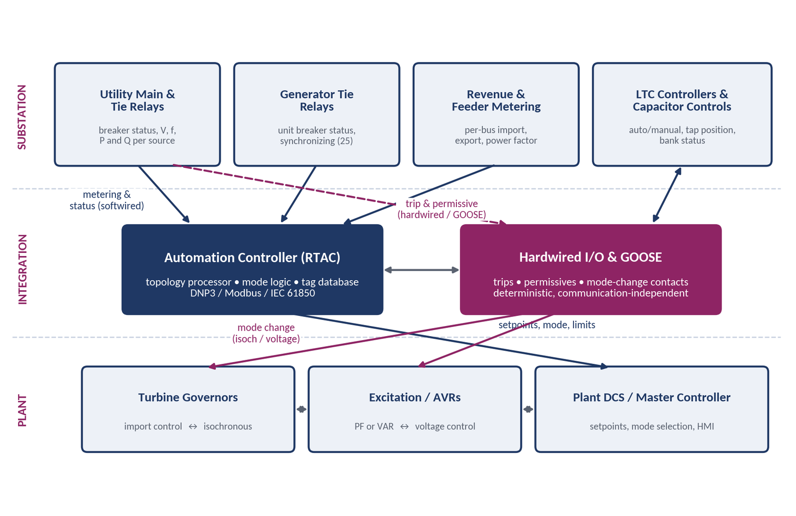
By SANDIP R PATEL
•
September 20, 2026
Learn CHP load following and island detection engineering for campus plants, including protection, controls, power studies, and grid transition design.
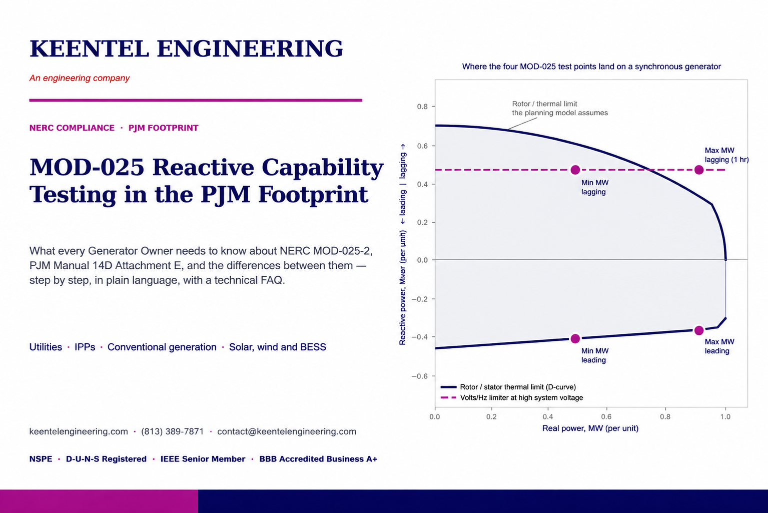
By SANDIP R PATEL
•
September 20, 2026
NERC MOD-025-2 Generator Owners, MOD-025-2 reactive power testing, generator capability verification, NERC Attachment 1, MOD-025 compliance testing
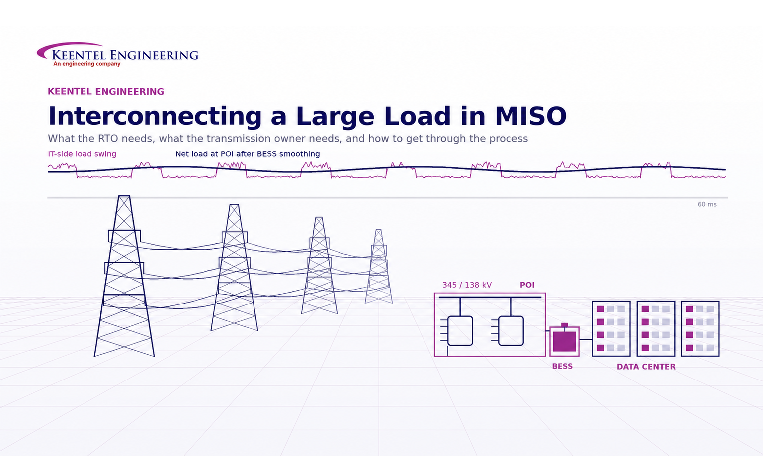
By SANDIP R PATEL
•
September 20, 2026
Understand MISO large load interconnection requirements for data centers, including TO data, PSS®E models, ride-through, harmonics, BESS and EPR.
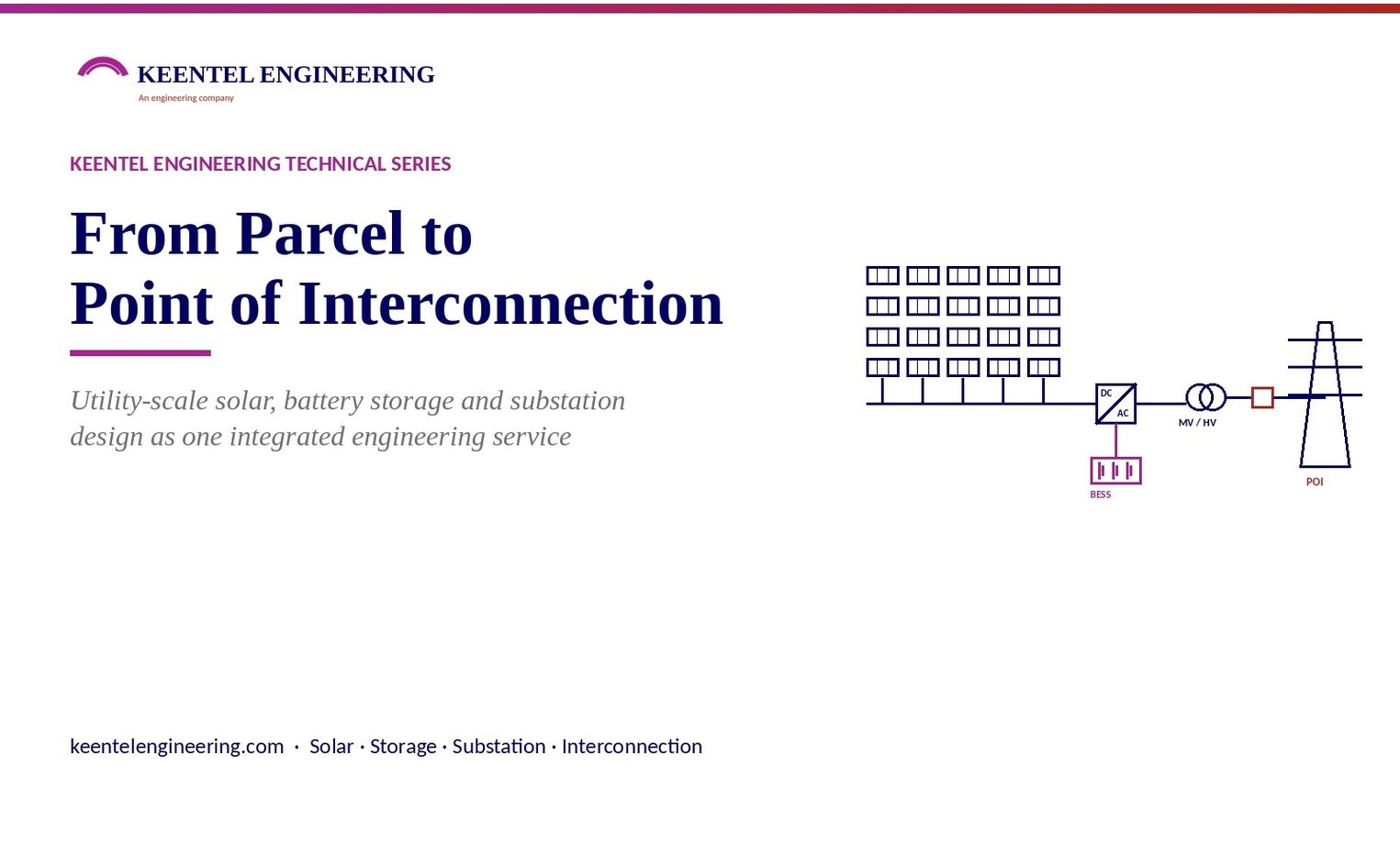
By SANDIP R PATEL
•
September 19, 2026
Explore utility scale solar engineering from site assessment to POI interconnection, including PV design, BESS, substation and grid studies.
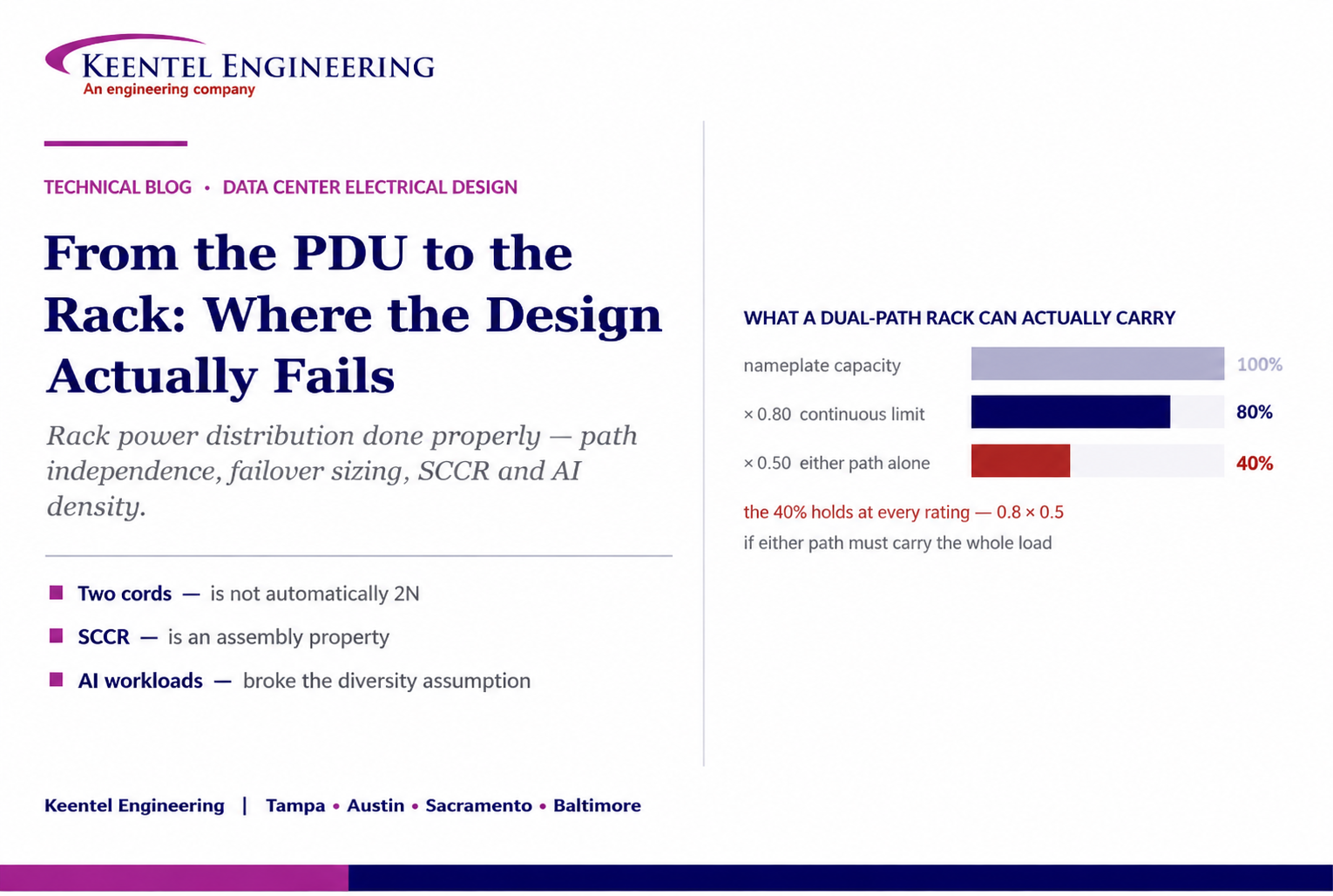
By SANDIP R PATEL
•
September 18, 2026
Learn how to size rack power distribution, PDU and RPP systems for continuous loads, A/B redundancy, failover capacity, SCCR and high-density AI data centers.

By SANDIP R PATEL
•
September 18, 2026
Learn why IP ratings like IP66, IP67, and IP68 do not tell the full story. Understand enclosure selection, NEMA differences, heat, corrosion, and protection.
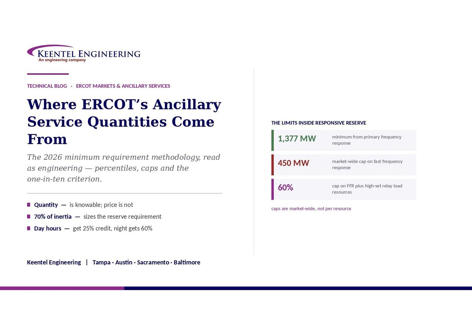
By SANDIP R PATEL
•
September 15, 2026
Learn how ERCOT calculates 2026 Regulation, RRS, ECRS and Non-Spin requirements, including inertia, FFR caps, forecast error and reserve methodology.