A Coordinated Electric System Interconnection Review—the utility’s deep-dive on technical and cost impacts of your project.
Challenge: Frequent false tripping using conventional electromechanical relays
Solution: SEL-487E integration with multi-terminal differential protection and dynamic inrush restraint
Result: 90% reduction in false trips, saving over $250,000 in downtime
ERCOT enforces all of the above through simulation, which means your model is your compliance case. The bar is now high:
- Whole-facility scope. The model must represent everything the IT load, the UPS and power conversion, the cooling plant, the protection and control systems in formats compatible with ERCOT's study platforms (PSS/E, PSCAD, TSAT).
- Real control loops, not approximations. Generic textbook representations are unacceptable. The model must capture the actual inner control behavior of your power electronics.
- Hardware-validated converter models. For electronic loads, the PSCAD model must be benchmarked against actual hardware testing including voltage ride-through and subsynchronous response. A model assembled from standard PSCAD library blocks fails by definition, because a generic block has never been tested against your vendor's hardware. The good news: validation is a hardware-type test, so results for a given converter product are reusable across every facility that uses it.
- Format migration. Facilities that previously submitted the older composite load model (CMLD) format must transition to EPRI's PERC1 format.
- Three checkpoints. Models are reviewed before the stability study begins (no model, no study), before each quarterly stability assessment, and for electronic loads one final time before energization, when you must submit as-built models with a documented comparison against the previously studied data and a sworn attestation that the model matches actual field settings. ERCOT's review takes 10 business days, extendable by 20 put it on your critical path.
- A living obligation. Change your technology, controls, or relay settings in a way that affects ride-through including converting a crypto mining site to an AI data center — and you've triggered a new interconnection study, even if your megawatts don't change.
| Parameter | Detail |
|---|---|
| System | 230 kV / 138 kV transmission corridors, wind and wet-snow icing exposure |
| Data basis | 15 years of minute-resolution forced-outage records + regional weather observations |
| Core methods | Event grouping, MVA performance curves, time-to-95%-restore, area outage rate curves, fragility modeling, rerun-history benefits, exceedance and log-domain risk metrics |
| Headline result | ≈85% of maximum resilience benefit at 60% of original capital; worst-event restoration window cut from 11 days to 5 in rerun-history terms |
| Decision supported | Capital portfolio selection; resilience plan filing; post-investment verification framework |
Grounding Analysis for Utility-Scale Solar Projects with WinIGS: An Integrated Engineering Approach

Jul 07, 2026 | Blog
A Keentel Engineering Technical Publication
Why Solar Plant Grounding Is Not a Bigger Substation Grid and Why the Software Choice Matters
A 100 MW solar plant occupies 500 to 900 acres. A transmission substation occupies five. Yet many grounding studies for utility-scale PV facilities still apply the mental model of the fenced substation yard — design a copper grid, check touch and step voltages inside the fence, stamp it, done. That model fails on solar plants, and it fails in ways that trace directly back to the analysis tool used.
Most grounding software analyzes a grounding system in isolation: the user draws the grid, enters a soil model, assumes a grid current, and the program computes potentials. WinIGS — the Windows-based Integrated Grounding System design program — is built on a fundamentally different premise: the grounding system is modeled together with the power system it belongs to. The network model (sources, transmission lines, transformers, collector circuits) and the geometric grounding model (conductors, rods, piles, fences, foundations) live in one integrated study case, and fault currents, split factors, and ground potential rise emerge from physics rather than from an input field. At Keentel Engineering, this is why WinIGS anchors our grounding practice for utility-scale solar: on a plant this electrically extensive, the assumed-grid-current shortcut is where studies go wrong before the first potential is ever computed.
Three realities of solar plants demand this integrated treatment.
First, the geographic extent changes the physics. A PV plant is not one grounding system; it is thousands of driven steel piles, hundreds of inverter and transformer pads, dozens of miles of medium-voltage collector circuits, a collector substation grid, perimeter fencing, and often a switchyard at the point of interconnection — all electrically interconnected and all embedded in soil that can vary by an order of magnitude across the site. The performance of any one element depends on all the others, and WinIGS's grounding model — built in a full 3-D geometric editor from electrode objects including ground rods, mats, bare and coated horizontal conductors, concrete foundations, and metallic fences — is designed to represent exactly that interconnected reality.
Second, the fault current picture is different. The worst fault for ground potential rise (GPR) at a solar collector substation is very often not a fault at the substation itself but a line-to-ground fault miles away, where the division of fault current between metallic return paths and the earth — the split factor — is least favorable. WinIGS's Maximum GPR analysis automates precisely this: it sweeps fault locations and types across the entire modeled network and identifies the worst fault, reporting its location, type, current, X/R ratio, and the resulting GPR. A study that begins with "assume the grid current is X kA" has already made its most consequential decision by assumption; a WinIGS study makes it by search.
Third, the design objectives multiply: personnel safety per IEEE Std 80 (or IEC 479-1 — both criteria sets are built into WinIGS), a stable reference for protection and communications, lightning protection per IEEE Std 998 via the program's integrated Lightning Shielding Analysis tool, and control of transferred potentials onto fences, pipes, and neighboring infrastructure.
Keentel Engineering's position is that grounding for utility-scale solar must be treated as an integrated, plant-wide power system study — grounding as a first-order design input, not a civil detail closed out at 90% design. WinIGS is the platform on which we execute that philosophy.
The Three-Standards Framework in WinIGS: Design, Verify, Shield
Our methodology organizes the study around three IEEE standards, and each maps onto specific WinIGS capability.
IEEE Std 80 — design criteria, computed natively.
WinIGS computes permissible touch, step, and metal-to-metal voltages directly from the study inputs: electric shock duration (from fault clearing time — we routinely evaluate backup clearing as well as primary), the soil resistivity model, the insulating surface layer thickness and resistivity, and the X/R ratio at the worst-fault location, from which the program derives the decrement factor for DC offset. The surface-layer reduction factor — crushed rock or asphalt derating — is computed to the IEEE Std 80-2000 formulation (the program retains older-edition options only for legacy-study compatibility). Because these inputs flow from the same integrated model that found the worst fault, the criteria and the stresses are always self-consistent.
IEEE Std 81 — measurement in, verification out.
On the front end, WinIGS ingests field soil data in all the standard forms — Wenner four-pin, Schlumberger, and driven-rod — and automatically estimates a two-layer soil model with statistical rigor: parameter tolerances at a user-set confidence level (90% default), a validity depth telling you how deep the survey can actually see, and graphical bad-data screening where outlier measurements are marked and excluded, visibly tightening the model tolerances. On the back end, WinIGS supports the verification workflow: its Point-to-Point Impedance analysis (Model B or D) predicts what continuity testing of the as-built system should measure, and its Smart Ground Meter integration allows field measurement locations to be imported and interface points generated automatically — closing the loop between model and measurement that IEEE 81 exists to enforce.
IEEE Std 998 — shielding in the same model.
The WinIGS Lightning Shielding Analysis tool implements all three IEEE 998 methods — the full electrogeometric model, the rolling sphere method, and the shielding angle method — operating directly on the same 3-D geometric model used for grounding: buildings, buswork, outdoor equipment, shield wires, and masts are modeled once and analyzed for both fault safety and stroke interception.
Design to 80, verify to 81, shield to 998 — one model, one tool, no re-entry of data between siloed programs.
Step 1: Soil Characterization Across a Heterogeneous Site
Everything rests on the soil model, and on a multi-hundred-acre site the biggest error we encounter in third-party studies is a single soil model extrapolated across the whole plant.
Our practice is to specify Wenner traverses at a density matched to site geology — several distributed across the array area plus dedicated sets at the collector substation and switchyard — with probe spacings pushed as far as logistics allow, because WinIGS's reported validity depth makes the limitation explicit: a survey with spacings to 100 feet supports a model to roughly 150 feet of depth and no further, and for an electrode the size of a solar plant, deep-layer resistivity governs.
Each traverse's data — either measured resistance or apparent resistivity; WinIGS accepts both and cross-computes the other, along with probe length and meter frequency — is processed through the program's soil interpretation engine, which fits the two-layer model and superimposes the fitted curve over the measured points. That plot is where field data quality becomes visible: measurements contaminated by buried metal or instrument error sit conspicuously off the curve, are marked as bad data with the Mark/Unmark function, and the re-run fit reports dramatically tighter parameter tolerances. A defensible soil model is one whose uncertainty is quantified, and this workflow quantifies it.
On sites with genuinely distinct soil regions — river terrace against upland clay, landfill cell against native ground — we model multiple conductor groups and soil regions rather than averaging site geology into a fiction that exists nowhere.
Step 2: The Integrated System Model in WinIGS
A WinIGS study case has two tightly coupled halves, edited in the program's two specialized environments.
The Network Editor
holds the power system as a single-line diagram: equivalent sources, transmission lines with their physical construction (conductor types and positions, tower geometry from the program's tower library, span length, structure footing resistance, shield wires), transformers including autotransformers with tertiaries, collector circuits, cable systems built from the cable library, and the grounding system elements that tie it all to earth. Our standard scope for a utility-scale PV model: the collector substation grid in full detail; the interconnecting transmission line modeled physically for the first several miles; equivalent sources at interface buses beyond; the 34.5 kV collector system with actual cable construction; representative inverter/transformer pads; the pile and racking network; and the perimeter fence.
Two modeling disciplines deserve emphasis. Equivalents must be verified, not assumed. The external network is reduced to equivalent sources and inter-bus equivalent circuits at the interface buses, with parameters taken from the utility's short-circuit model (ASPEN, CAPE, or similar). The acceptance test is non-negotiable: the reduced WinIGS model must reproduce the utility's fault duties at the POI before any grounding conclusion is drawn. Exact match is not expected — WinIGS's physically based three-phase models capture asymmetries that classical short-circuit programs ignore — but the discrepancy must be quantified and small. Everything needs a path to remote earth, and everything conductive is part of the answer. WinIGS enforces the first as a modeling rule (a floating delta tertiary will stop the solver, for good reason); the second is engineering judgment the tool supports: reinforced-concrete foundations are modeled as steel mat electrodes on a dedicated Foundations layer — capturing their Ufer-effect contribution while WinIGS's layer system keeps them out of the auto-generated Bill of Materials, since they're structure, not purchased copper.
The Ground Editor
holds the physical grounding model in true 3-D — top, side, perspective, and rendered views — with the site's foundation drawing imported as a scaled background image (DXF import/export is supported for CAD interchange), so grounding conductors are placed against real equipment locations, not idealized rectangles. Analysis model fidelity is selectable: Model A for rapid equipotential-conductor screening through Models B, C, and D, which represent voltage drop along conductor lengths — with the enhanced Model C in current releases capturing ground-conductor self-inductance at near-Model-D accuracy for a fraction of the runtime, a meaningful advantage on plant-scale models with thousands of electrode segments.
Step 3: Worst-Fault Search and Split Factor the Maximum GPR Analysis
With the model built, WinIGS's Maximum GPR analysis runs a large automated series of fault simulations — every fault type, swept along every line and bus within a user-set radius (or the whole system) — and identifies the fault producing maximum GPR at the monitored node. The report is the design basis in one screen: worst fault type and location, fault current magnitude and phase, X/R at the fault, and the GPR.
Three phenomena make this search essential on solar plants. The split factor — reported directly in WinIGS's Ground Resistance report as the ratio of earth current to fault current — varies strongly with fault location, and the worst case is routinely a fault out on the line, not at the station. Transformer winding effects are captured physically: WinIGS's Internal I/O reporting shows the circulating current in a delta tertiary during ground faults — a current that can exceed 10 kA while the winding's terminal currents read zero, and that raises GPR for remote faults while lowering it for local ones. And on the collector side, the grounding-source configuration for the 34.5 kV system shapes touch voltage at every inverter pad in the plant.
Typical well-designed collector substations on effectively grounded transmission systems see split factors in the 20–40% range. An isolated-grid study assuming 100% of fault current enters the earth over-designs by a factor of three to five; one that guesses low gambles with compliance. WinIGS replaces the guess with a computation.
Step 4: Safety Assessment — Touch, Step, and Transferred Potentials
Against the worst-fault condition, WinIGS computes earth-surface potentials and evaluates touch and step voltages over user-defined assessment regions rectangular or polygonal plot frames drawn directly on the grounding model. Region definition is engineering judgment the tool makes explicit: touch-voltage frames cover everywhere a person can stand and reach grounded metal — substation interior plus a band extending three feet outside the fence, every inverter pad and enclosure row; step-voltage frames emphasize the areas just outside perimeter fences where gradients peak; and each frame is assigned its own permissible basis crushed-rock derating inside the station, native-soil criteria in the arrays and beyond the fence.
The results read as color-coded equipotential contour plots with the maximum location flagged and the permissible value printed alongside compliance or violation at a glance plus a rendered 3-D touch-voltage surface where violations rise as literal red peaks above the plant. Those peaks are a design instruction: they show precisely where conductor must be added, which is a far more economical process than uniformly densifying the grid. Two referencing details matter for correctness at plant scale, and WinIGS handles both: touch voltage referenced to the nearest grounding point (the recommended setting for Models B/C/D, where conductor voltage drop is represented) rather than a single remote reference; and step voltage computed across the standard 3-foot stride distance.
Transferred potential closes the assessment. WinIGS's user-defined contour feature draws the zone-of-influence boundary commonly the 300 V contour directly on the site plot, making visible which pipelines, fences, communication routes, and neighboring facilities fall inside it during the worst fault and therefore require isolation, gradient control, or dedicated mitigation.
Step 5: Design Enhancement — Where the Money Is
The study is complete when the as-built system is measured and reconciled. Our commissioning scope: fall-of-potential impedance measurement with leads long enough to escape the zone of influence WinIGS plotted; plant-wide continuity verification, with WinIGS's Point-to-Point Impedance report generating the predicted value for every test-point pair — the complete pairwise report exports to file for direct comparison against field data; and investigation of every divergence before energization. A measured point-to-point impedance that disagrees with the model is not noise — it is a missing bond, a broken conductor, or a soil surprise, found while it is still cheap to fix.
WinIGS is a proprietary software product of its respective developer and owner. Keentel Engineering is an independent consulting engineering firm and is not affiliated with, endorsed by, or sponsored by the developers of WinIGS or any other software vendor or standards organization referenced herein. IEEE Std 80, IEEE Std 81, and IEEE Std 998 are publications of the Institute of Electrical and Electronics Engineers. All product names and trademarks are the property of their respective owners.
Case Study
Case Study 1: 120 MW PV Plant — Three Bonding Strategies Settled by One WinIGS Model
Situation
A utility-scale PV facility in the southeastern U.S. — roughly 120 MW across approximately 700 acres, 34.5 kV collection, 115 kV interconnection — engaged Keentel to resolve a design dispute between the EPC and the owner's independent engineer over array bonding philosophy: (A) isolated array grounding, each inverter block grounded locally and deliberately not bonded to the collector substation; (B) fully integrated bonding tying racking, pads, and station into one continuous system; (C) a hybrid integrating the collector grounding while insulating fence sections remote from the substation.
Approach
Rather than argue philosophy, we built one WinIGS integrated study case and ran all three schemes as variants of it. The Network Editor model carried the 115 kV interconnection with shield wires and structure grounds, equivalent sources tuned until the reduced model reproduced the utility's fault duties at the POI, the full collector system with actual cable construction, and the BESS-ready station arrangement; the Ground Editor model carried the station grid, pads, pile network, and fencing over the imported site drawing. Fourteen Wenner traverses were processed through the soil interpretation engine — site resistivity ranged from about 90 Ω·m over 30 Ω·m in the bottomland to over 400 Ω·m in the upland third, so two soil regions were modeled with separate conductor groups rather than averaged. The Maximum GPR analysis was run for each variant against both transmission and collector systems.
Findings
The isolated scheme (A) — defended as preventing station GPR from "exporting" into the arrays — performed worst. The model showed the isolation to be largely fictional (cable neutrals and incidental paths defeat it), while depriving inverter pads of the gradient control the integrated network provides: during the worst collector-side fault, the touch-voltage plot frames at three pads showed exceedances over 40% above the native-soil permissible. The integrated scheme (B) cleared the pad violations and cut station impedance by roughly a third — the pile network's contribution, now visible in the Ground Resistance report — but the transmission-side worst fault transferred elevated potential onto remote fence runs, and the fence-line frames lit up nearly half a mile from the station. The hybrid (C) met criteria everywhere: integrated bonding delivered the pad safety and impedance benefit, insulated fence breaks with local gradient loops handled the remote transfer.
Outcome
Scheme C became the grounding design basis. The quantified pile contribution supported a reduction of the station grid from the EPC's preliminary layout, offsetting most of the fence-mitigation cost. At commissioning, point-to-point continuity results matched WinIGS predictions across the test-point set, and the fall-of-potential measurement of the completed system landed within 12% of the model's computed impedance.
Case Study 2: High-Resistivity Mountain Site — WinIGS Split-Factor Analysis Beats a Copper Crisis
Situation
A 150 MW solar project in mountainous western-U.S. terrain hit a grounding crisis at 60% design: shallow soil over rock, survey models showing 600–1,100 Ω·m upper layers, and an EPC study — an isolated-grid analysis with an assumed grid current — concluding that compliance required massive grid densification plus deep wells at a cost the project could not absorb.
Approach
Keentel rebuilt the problem in WinIGS as an integrated study. The 230 kV interconnection was modeled physically for the first several miles — both shield wires, tower geometry from the tower library, measured footing resistances — with the external network reduced to equivalent sources and inter-bus equivalents verified against the utility's short-circuit duties at the POI. The Maximum GPR analysis, searching all fault locations, placed the governing fault on the 230 kV line roughly a mile and a half from the plant — and the Ground Resistance report put the split factor near 25%: only about a quarter of the fault current actually entered the earth at the station. The EPC study's assumed grid current had been more than triple physical reality.
Findings
With the computed earth current, the crisis shrank but did not vanish: touch-voltage frames along one switchyard edge still showed exceedances around 20%, and the station GPR kept a fiber route and a pipeline crossing inside the 300 V zone-of-influence contour WinIGS plotted on the site plan. Two mitigations were engineered in the same model. Grid enhancement needed on the order of 1,300 additional feet of 4/0 in rock trench — and the re-run showed GPR essentially untouched, leaving the transferred-potential exposures alive. The counterpoise alternative used the Model Conversion tool to convert the first two spans to the mutually coupled multiphase line model, adding a buried counterpoise conductor bonded to structure grounds and the station grid through a corridor of deeper soil. Result: station GPR down approximately 25%, every touch frame under permissibles with better than 10% margin, the 300 V contour pulled inside the pipeline crossing — at under two-thirds the conductor length of the copper-only option, in trenchable soil.
Outcome
The counterpoise design was built. Total grounding cost came in below half the EPC's original mitigation estimate, and the study package — worst-fault basis, split-factor derivation, soil model with confidence tolerances, IEEE 81 verification plan — cleared utility review on first submittal. On hard-soil sites, the cheapest copper is the copper the split-factor computation proves you don't need.
Case Study 3: Solar-Plus-Storage Collector Station — the Worst Fault Wasn't Where Anyone Looked
Situation
A solar-plus-storage facility — approximately 200 MW PV with a 100 MW / 400 MWh BESS sharing the collector substation — engaged Keentel after the owner's engineer flagged that the preliminary grounding study had evaluated only station bus faults. The station was electrically busy: two 34.5 kV collector buses, a BESS medium-voltage system with its own grounding transformer, a main transformer with a buried delta tertiary, and a 138 kV interconnection.
Approach. The WinIGS model carried the full station, the 138 kV line with shield wires, and both feeder systems with their distinct grounding sources; the delta tertiary was modeled explicitly (with its required path to remote earth). The Maximum GPR analysis was configured with the search radius at zero — every circuit, transmission and medium-voltage alike — and the tertiary's behavior was examined via Internal I/O reports under both remote and local fault cases.
Findings
The governing fault was a line-to-ground fault on a 34.5 kV BESS feeder a short distance from the station — not the 138 kV bus fault the preliminary study assumed conservative. Two effects an isolated study cannot see drove it. The BESS grounding transformer fed ground-fault current returning through station earth for close-in feeder faults, over a cable system whose metallic return was weaker than the transmission side's shield wires — an unfavorable split, visible directly in the split-factor output. And the delta tertiary, inert at its terminals, circulated over 10 kA in the Internal I/O report during the feeder fault, adding to the earth current for that case while reducing GPR for the bus-fault case — the exact inversion of the preliminary study's assumption. Touch-voltage plot frames around the BESS enclosure rows, evaluated against the feeder fault with the decrement factor from that location's X/R, showed exceedances at eleven enclosure positions.
Outcome
Mitigation was surgical: gradient-control loops around the affected rows, a revised neutral-grounding-resistor specification for the BESS grounding transformer that trimmed fault contribution without degrading protection sensitivity, and one relocated feeder ground bond roughly 900 feet of added conductor per the final Bill of Materials, versus the several-thousand-foot blanket densification a bus-fault-only reading would have driven. At commissioning, WinIGS's exported point-to-point impedance predictions exposed one unbonded BESS enclosure row construction had missed — the measured value disagreed with the model, and the model was right. The station has since cleared two real collector-system ground faults without incident.
Frequently Asked Questions
1. What makes WinIGS different from conventional grounding-grid software?
The integration. Conventional tools analyze a grounding grid in isolation and require the user to assume the grid current — the single most consequential number in the study. WinIGS models the grounding system together with the surrounding power system (lines, sources, transformers, collector circuits) in one study case, so fault current, split factor, and GPR are computed results of a network solution, not inputs. On a geographically extensive solar plant, where the worst fault is usually remote and the metallic return paths are complex, that difference is decisive.
2. What is the split factor, and where does WinIGS report it?
The split factor is the ratio of current actually entering the earth through your grounding system to the total fault current; shield wires, cable neutrals, and counterpoises carry the rest back metallically. WinIGS reports it directly in the Ground Resistance report alongside grid impedance and the per-group earth currents. Because compliance scales with earth current, a study assuming 100% when the true split is 30% forces roughly triple the copper the site needs — or, erring the other way, delivers a non-compliant plant with a compliant-looking report.
3. How does the Maximum GPR analysis find the worst fault?
It automates a fault sweep: line-to-ground and line-to-neutral faults are simulated at the buses and along the length of every circuit in the model (optionally limited to a radius around the monitored node; set the radius to zero to search everything), and the program reports the fault that maximizes GPR at your grounding system — location, type, current, and the X/R ratio at that location, which WinIGS then uses for the decrement factor in the permissible-voltage computation. The worst fault on solar interconnections is routinely a transmission-line fault one to two miles out, or a close-in collector feeder fault — locations no bus-fault-only study ever examines.
4. What soil data does WinIGS accept, and how does it handle measurement error?
Wenner (four-pin), Schlumberger, and driven-rod data, entered as either measured resistance or apparent resistivity — the program cross-computes the other — along with probe length and meter frequency. It fits a two-layer soil model and reports each parameter with a tolerance at a user-set confidence level, plus a validity depth stating how deep the survey can actually resolve. Outliers are visible against the fitted curve, are excluded with the Mark/Unmark function, and the re-fit shows the tolerance improvement. That statistical transparency is what makes the soil model defensible in front of a reviewing utility.
5. IEEE Std 80 or IEC 479-1 — which does WinIGS apply?
Both criteria sets are built in; the user selects per project. For North American utility-scale solar, IEEE Std 80 is the near-universal basis, with the surface-layer reduction factor computed to the Std 80-2000 formulation. The shock-duration input should be a documented decision reflecting realistic clearing times — we evaluate backup clearing as a sensitivity, because a design with zero margin against a stuck breaker depends on perfection.
6. Can WinIGS model the PV racking piles as grounding electrodes?
Yes — driven piles, racking bonds, and equipment grounding conductors are modeled with the standard electrode objects, and this matters enormously: thousands of individually mediocre electrodes form a distributed network whose aggregate contribution often rivals the deliberate copper. Our practice is to model the pile network realistically, credit it conservatively in design decisions, keep structural elements on separate layers so the Bill of Materials reflects only purchased conductor, and verify the bonding assumptions at commissioning via point-to-point testing.
7. What are WinIGS analysis Models A, B, C, and D, and which should a solar study use?
They are ascending fidelity levels for the grounding solution. Model A treats conductors as equipotential — fast, fine for early screening. Models B, C, and D represent voltage variation along conductors, which matters on plant-scale systems where a "grounded" structure half a mile from the station is not at station potential; the current enhanced Model C captures conductor self-inductance at near-Model-D accuracy with substantially less runtime. For final safety assessment on large plants we use Model B at minimum, with the nearest-grounding-point touch reference — the recommended setting for these models.
8. How does WinIGS handle the delta tertiary on the main power transformer?
Physically. The autotransformer-with-tertiary model carries the winding in the network solution, and the Internal I/O report displays its circulating current — which can exceed 10 kA during ground faults even while terminal currents read zero. The tertiary raises GPR for faults outside the station and reduces it for local faults, so a study that ignores it (or a solver that can't represent it) mis-ranks the fault cases. Note WinIGS's modeling rule that every winding needs a path to remote earth — a floating delta is tied to the neutral system through a phase-terminal connector, or the solver will rightly refuse to run.
9. High GPR but compliant touch voltages — is that a problem?
It is a different problem. GPR is the grid's rise relative to remote earth; touch voltage is the local difference a person actually experiences, and a well-graded grid keeps that small even at several kV of GPR. High GPR is primarily a transferred-potential issue — communications isolation, pipelines, fences leaving the site. WinIGS's user-defined contour (typically 300 V) draws the zone of influence on the site plan so every exposure inside it is identified and mitigated, and if the zone must shrink, counterpoise — which cuts the earth current itself — is the lever.
10. Counterpoise or more grid copper — how do we decide?
Model both against the same worst fault and read the two Bills of Materials. Local touch violations with acceptable GPR → targeted conductors at the red peaks on the 3-D touch surface. Elevated GPR with broad violations or transferred-potential exposure → counterpoise on the interconnecting line, built in WinIGS by converting the line to the mutually coupled multiphase model and adding the below-grade conductor. In our project experience the counterpoise frequently wins on installed cost — especially in rock — because it reduces the earth current every other measure is fighting.
11. How does WinIGS support IEEE 81 field verification?
Three ways. The soil interpretation engine is the front end for the IEEE 81 resistivity survey. The Point-to-Point Impedance analysis (Model B or D) predicts the value every continuity test of the as-built system should measure, and exports the complete pairwise report for comparison against field results. And Smart Ground Meter integration imports measurement locations and auto-generates the corresponding interface points in the model. Verification is the difference between a hypothesis and an engineering deliverable; the tool is built to close that loop.
12. Does the lightning shielding analysis require a separate model?
No — that is much of its value. The Lightning Shielding Analysis tool runs on the same 3-D geometric model as the grounding study, using rolling sphere, shielding angle, or the full electrogeometric method per IEEE 998. Equipment, buswork, masts, and shield wires are modeled once; shielding gaps are fixed by editing the same layout the grounding conductors live in, and the down-conductor earthing is evaluated in the same soil model. One geometry, both physics.
Q. What is resilience-adjusted capacity value (resilience-adjusted ELCC)?
An extension of effective load carrying capability into extreme-event conditions. A resource is evaluated across a probability-weighted set of disruptive scenarios, each with its own intensity, duration, and restoration trajectory; the metric is the probability-weighted fractional reduction in expected energy not served that the resource delivers. Multiplying by VoLL and representative event duration converts it into avoided outage cost — letting storage, generation, DERs, and wires-based hardening compete in a single valuation framework.
Q. What does it mean that blackout costs are "heavy-tailed," and why should I care?
Empirical exceedance curves of event customer cost on real distribution systems show log-log tail slopes with magnitude below one — an extremely heavy tail. Practically: there is no "typical" large blackout, large events dominate total risk, and sample means over the tail do not converge with available data. That invalidates expected-value tools, including conditional value-at-risk and expected-cost optimization, for large-blackout risk. The defensible alternatives are exceedance metrics (probability and annual frequency of exceeding a cost threshold) and log-domain indices that average the logarithm of large-event costs.
Q. Which resilience metrics do regulators actually respond to?
Metrics that are computable from recorded data, auditable, and expressible in customer terms: customer-hours lost per event, restoration times to defined percentiles, critical-facility continuity, frequency of large-cost events, and avoided-cost figures with transparent VoLL or damage-function assumptions. Composite indices are useful for communicating trends, but filings are won on the underlying independent metrics and the traceability of the analysis behind them.
Q. Should we aggregate everything into one resilience score?
Generally no. Independent metrics for distinct resilience attributes — robustness, absorption, restoration speed, customer impact, cost — preserve the diagnostic information that drives investment decisions. Where a single score is genuinely required, use dynamic aggregation in which component weights vary with event type and contingency level, and always publish the components alongside the composite.
Q. How do transmission and distribution resilience metrics differ?
Transmission metrics emphasize energy not served in MWh, stability margins, N-k withstand, topological criticality, and cascading exposure, computed from SCADA and synchrophasor data with detailed dynamic models. Distribution metrics emphasize customers interrupted, customer-hours, restoration rates, critical-load continuity, and reconfiguration or islanding capability, computed from outage management and AMI data. A sound framework aligns both on shared dimensions — restoration duration, robustness, recovery slope — so results compare across the hierarchy.
Q. What resilience metrics apply to microgrids and islandable systems?
Sustainable islanding duration under realistic resource and load profiles; fraction of critical and total demand met by local resources; voltage and frequency stability in islanded operation; transition success rate and speed between grid-connected and islanded modes; and the support the system can provide to the wider grid during emergencies. For community systems, these are typically paired with critical-facility continuity metrics for hospitals, water, communications, and shelters.
Q. How do crew and logistics factor into resilience measurement?
Through restoration-effort metrics: crew deployment tracked hourly through an event yields total crew-hours; customer-hours restored per crew-hour measures restoration efficiency; crew-hours per outage restored measures crew effectiveness; and a logarithmic composite of average customer restoration duration and crew-hours per outage gives a single emergency-response efficiency score comparable across events of different sizes. These metrics turn staffing, staging, and mutual-assistance decisions into quantitative questions.
Q. Can existing reliability metrics be adapted for resilience?
Yes, by threshold conditioning: restrict the metric to events exceeding a severity criterion — duration beyond 24 hours, more than a set number of simultaneous outages, or cost above a defined level. Threshold-conditioned load-curtailment and energy-not-served metrics reuse existing data pipelines and institutional familiarity, and are often the fastest route to a defensible resilience baseline.
Q. What role do AI, IoT, and real-time monitoring play?
Machine learning supports failure prediction, vegetation and asset risk scoring, damage forecasting ahead of storms, and restoration optimization. Dense IoT sensing and synchronized measurements raise system observability, enabling real-time resilience metric evaluation during events rather than only post-event reconstruction. These technologies strengthen every lifecycle phase — but they inherit the data-quality and cyber-security obligations that come with expanded digital surface area.
Q. Where should a utility or developer start?
With a baseline: extract resilience events from the last five to ten years of outage records, compute the core event metrics (size, customer-hours, restoration percentile times, nadir), build the cost exceedance curve, and identify the two or three hazard types that dominate the tail. That baseline scopes everything downstream — which hardening options to model, which scenarios to simulate, and what a credible avoided-cost case looks like. It is typically a focused engineering effort measured in weeks, not a multi-year program.

About the Author:
Sandip "Sonny" R. Patel, P.E.
IEEE Senior Member · Founder & CEO, Keentel Engineering
In 1995, Sonny Patel earned his Electrical Engineering degree from the University of Illinois. But degrees don't build legacies — action does.
For three decades, he has worked the power industry from every side of the table: 16 years as a utility engineer at Exelon/Commonwealth Edison; generation leadership across hydroelectric, industrial steam turbine, and a 9 GW renewable fleet; NERC Regional Entity Senior Compliance Engineer and Audit Team Lead, auditing some of the nation's largest utilities; and testing and commissioning lead on equipment up to 765 kV — the very top of the North American grid.Utility. Generator. Regulator. Consultant. Few engineers have seen all four seats. Fewer still have sat in them.
His experience spans nuclear, hydro, conventional generation, renewables, oil and gas, mining — and today's data centers, where he is authoring a three-book series on data center design. He is a Licensed Professional Engineer in six states and a Licensed Electrical Contractor in Florida (Unlimited EC) — he doesn't just design the work; he's qualified to stand behind its execution.Today, as Founder and CEO of Keentel Engineering, Sonny leads a nationwide team of engineers delivering substation design, power system studies, NERC compliance, and commissioning — done right, coast to coast.Three decades. Every side of the table. One standard: accountable engineering.
Services

Let's Discuss Your Project
Let's book a call to discuss your electrical engineering project that we can help you with.
About the Author:
Sandip "Sonny" R. Patel, P.E.
IEEE Senior Member · Founder & CEO, Keentel Engineering
In 1995, Sonny Patel earned his Electrical Engineering degree from the University of Illinois. But degrees don't build legacies — action does.
For three decades, he has worked the power industry from every side of the table: 16 years as a utility engineer at Exelon/Commonwealth Edison; generation leadership across hydroelectric, industrial steam turbine, and a 9 GW renewable fleet; NERC Regional Entity Senior Compliance Engineer and Audit Team Lead, auditing some of the nation's largest utilities; and testing and commissioning lead on equipment up to 765 kV — the very top of the North American grid.
Utility. Generator. Regulator. Consultant. Few engineers have seen all four seats. Fewer still have sat in them.
His experience spans nuclear, hydro, conventional generation, renewables, oil and gas, mining — and today's data centers, where he is authoring a three-book series on data center design. He is a Licensed Professional Engineer in six states and a Licensed Electrical Contractor in Florida (Unlimited EC) — he doesn't just design the work; he's qualified to stand behind its execution.
Today, as Founder and CEO of Keentel Engineering, Sonny leads a nationwide team of engineers delivering substation design, power system studies, NERC compliance, and commissioning — done right, coast to coast.Three decades. Every side of the table. One standard: accountable engineering.
Leave a Comment
Thank you for contacting us.
We will get back to you as soon as possible.
We will get back to you as soon as possible.
Oops, there was an error sending your message.
Please try again later.
Please try again later.
Related Posts
By SANDIP R PATEL
•
October 3, 2026
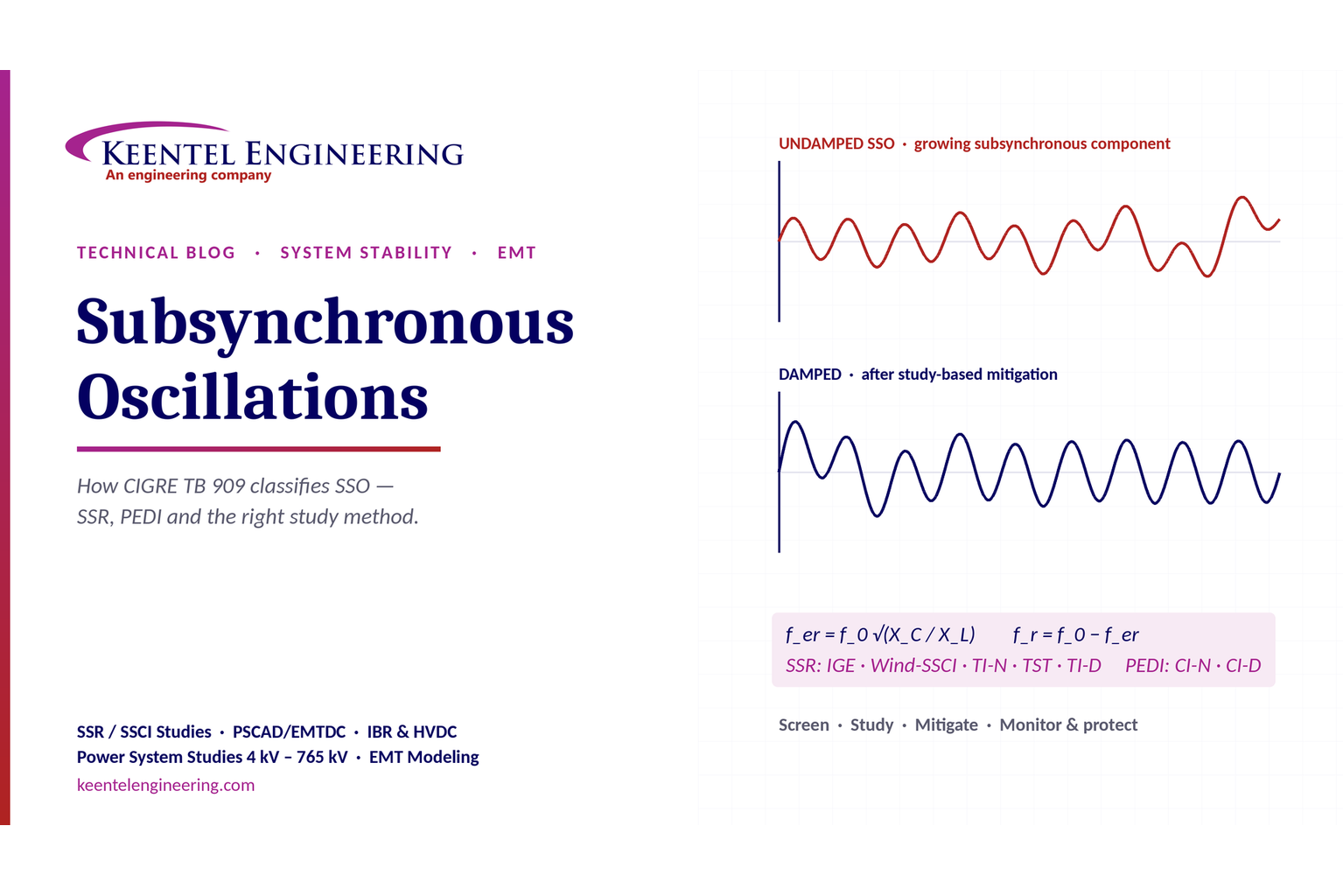
A practical guide to SSO classification, SSR, PEDI, Wind-SSCI, EMT analysis, mitigation and protection based on CIGRE TB 909.
By SANDIP R PATEL
•
October 3, 2026
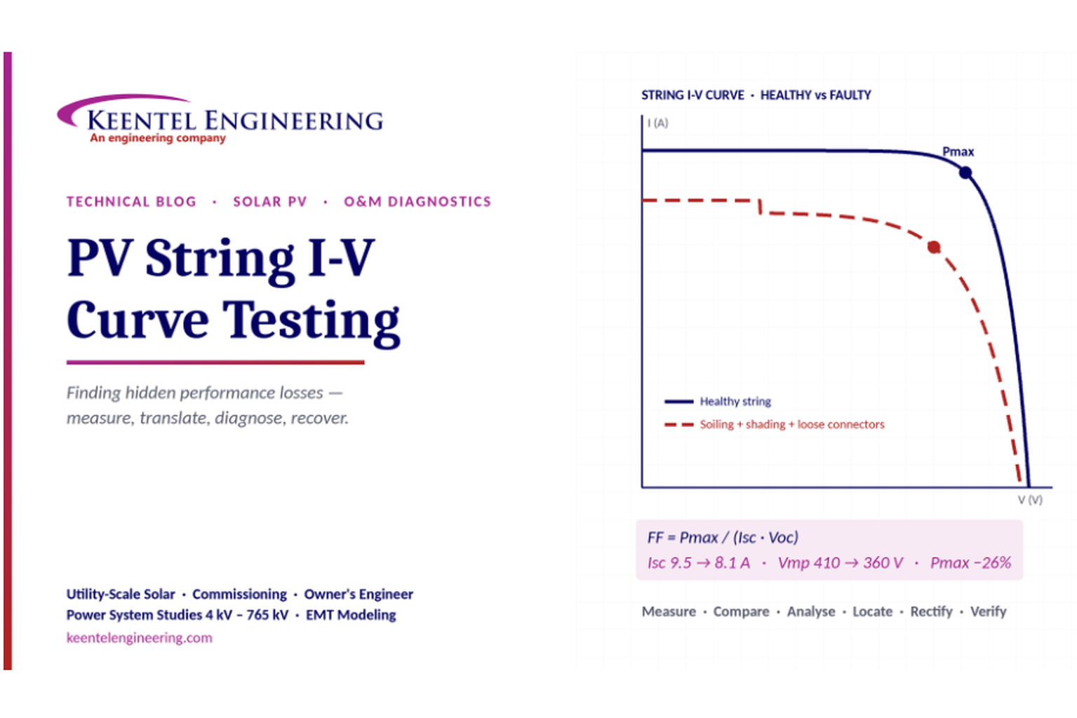
Learn how PV string I-V curve testing identifies hidden solar performance losses, including soiling, shading, mismatch, degradation, and wiring faults.
By SANDIP R PATEL
•
October 3, 2026
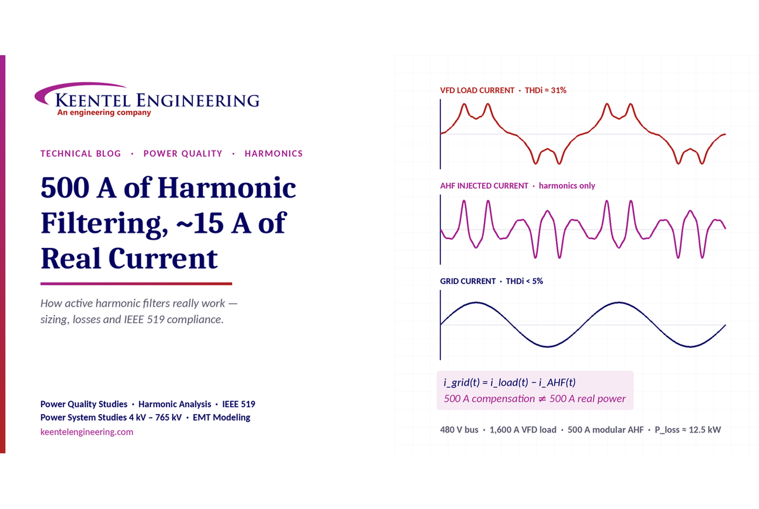
Learn how active harmonic filters work, how to size AHF systems, reduce VFD harmonics, calculate losses, and meet IEEE 519 TDD limits at the PCC.
By SANDIP R PATEL
•
October 3, 2026
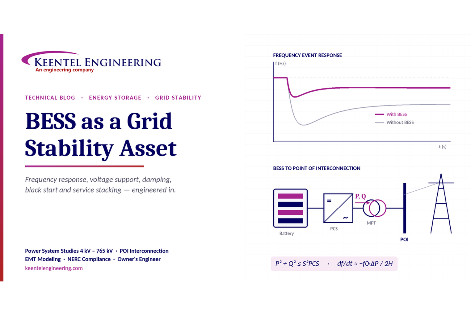
Learn how BESS supports grid stability through fast frequency response, voltage support, oscillation damping, black start, grid-forming controls and EMT studies.
By SANDIP R PATEL
•
September 30, 2026
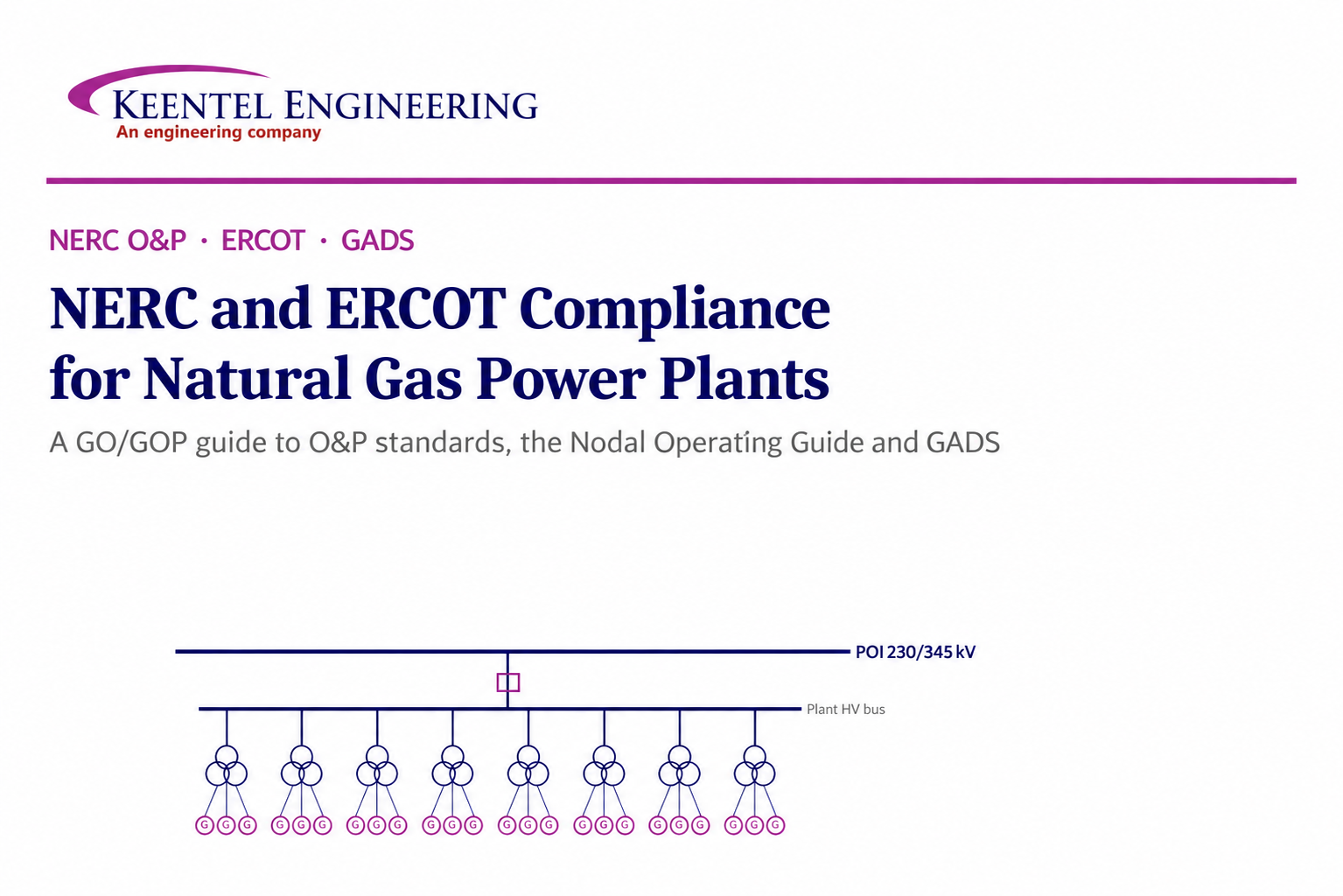
Learn NERC and ERCOT compliance requirements for natural gas power plants, including GO/GOP obligations, O&P standards, GADS reporting, and audits.
By SANDIP R PATEL
•
September 26, 2026
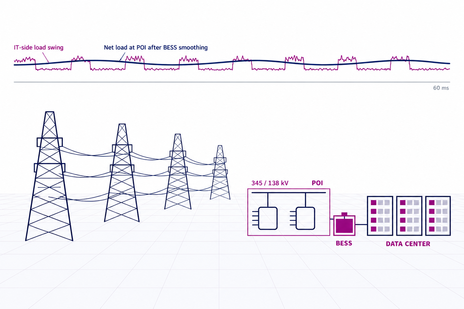
Learn how to prepare a MISO large-load interconnection package, including PSS®E models, BESS smoothing, harmonic data and transmission-owner requirements.
By SANDIP R PATEL
•
September 26, 2026
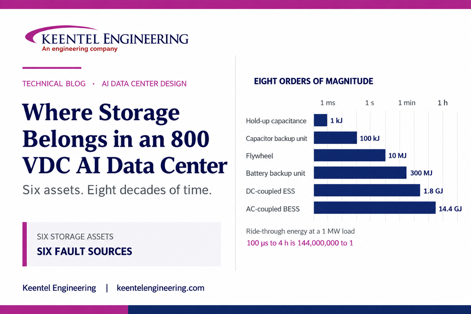
Learn where storage belongs in an 800 VDC AI data center, including capacitors, flywheels, BESS, fault current, protection, grounding, and EMT design.
By SANDIP R PATEL
•
September 26, 2026
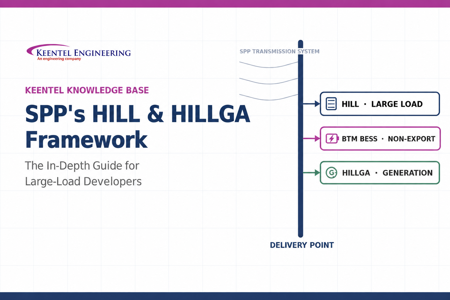
Learn how SPP’s HILL and HILLGA framework works for large-load projects, including studies, BTM generation, modeling, EMT requirements, and firm service.
By SANDIP R PATEL
•
September 25, 2026
Learn how IBR time synchronization, IEEE 2800, IRIG-B verification, and PTP solutions help meet disturbance monitoring compliance requirements.